
Click to learn more about author Rosaria Silipo.
The co-authors of this column were Kathrin Melcher and Maarit Widmann.
The Fraud Detection Problem
Fraud detection belongs to the more general class of problems — the anomaly detection. Anomaly is a generic, not domain-specific, concept. It refers to any exceptional or unexpected event in the data, be it a mechanical piece failure, an arrhythmic heartbeat, or a fraudulent transaction as in this study. Indeed, to identify a fraud means to identify an anomaly in the realm of a set of legitimate “normal” credit card transactions. Like all anomalies, we are never sure of the form a fraudulent transaction will assume. We need to be prepared for all possible “unknown” forms.
There are two main approaches to fraud detection.
- Based on the histograms or on the box plots of the input features, a threshold can be identified. All transactions with input features beyond that threshold will be declared fraud candidates (discriminative approach). Usually, for this approach, a number of fraud and legitimate transaction examples are necessary to build the histograms or the box plots.
- Using a training set of just legitimate transactions, we teach a machine learning algorithm to reproduce the feature vector of each transaction. Then we perform a reality check on such a reproduction. If the distance between the original transaction and the reproduced transaction is below a given threshold, the transaction is considered legitimate; otherwise it is considered a fraud candidate (generative approach). In this case, we just need a training set of “normal” transactions, and we suspect an anomaly from the distance value.
In order to be prepared for all unexpected events, we decided to adopt this second approach in our fraud detection project.
In this example, we use credit card data provided by Kaggle. The data set contains credit card transactions performed in September 2013 by European cardholders.
The transactions have two labels: “1” for fraudulent and “0” for normal transactions. The total number of transactions is 284,807. Only 492 (0.2 percent) of them are fraudulent. Each credit card transaction is represented by 30 features: 28 principal componentsextracted from the original credit card data, the time between each transaction and the first transaction in the data set, and the amount paid for each transaction.
Notice that, for privacy reasons, the data contains principal components instead of the original transaction features. You could, of course, use any other normalized, numeric features for this case study on fraud detection.
The Autoencoder Architecture
Many machine learning algorithms could be used to reproduce the vector of features representing a credit card transaction. One technique in particular is very well suited for this task and has been successfully used for this kind of problem: the neural autoencoder. (See, for example, Abel G. Gebresilassie’s “Neural Networks for Anomaly (Outliers) Detection,” but there are many more examples of using neural autoencoders for anomaly detection.)
An autoencoder is a feed-forward multilayer neural network that reproduces the input data on the output layer. By definition then, the number of output units must be the same as the number of input units. The autoencoder is usually trained using the backpropagation algorithm against a loss function, like the mean squared error (MSE).
Figure 1 shows the architecture of a simple autoencoder with only one hidden layer, as introduced in this video, “Neural networks [6.1]: Autoencoder – definition,” by Hugo Larochelle. More complex autoencoder architectures include additional hidden layers.
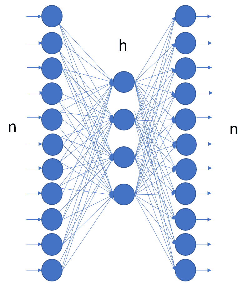
Figure 1: Structure of an autoencoder with one input layer with n units, one output layer also with n units, and one hidden layer with h units. The autoencoder is a feedforward network and is trained, usually with backpropagation, to reproduce the input vector onto the output layer.
For this case study, we built an autoencoder with three hidden layers, with the number of units 30-14-7-7-30 and tanh and reLu as activation functions, as first introduced in the blog post “Credit Card Fraud Detection using Autoencoders in Keras — TensorFlow for Hackers (Part VII),” by Venelin Valkov.
The autoencoder was then trained with Adam — an optimized version of backpropagation — on just legitimate transactions, for 50 epochs, against the MSE as a loss function.
Rule for Fraud Candidates

Data Preparation
There is not much to do for data preparation in this use case, just a few steps.
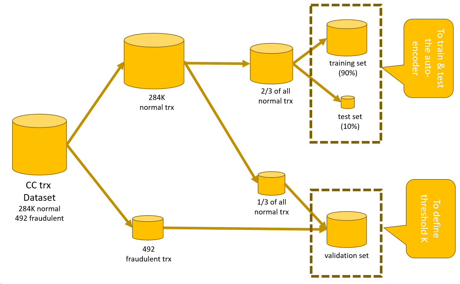
Figure 2: Data sets used for the anomaly detection process. First we exclude all fraudulent transactions from the original data set. With the remaining fraudulent transactions and some legitimate transactions, we build a validation set. From the “all normal transactions” data set, we create the training and test set to train and test the autoencoder.
- Split the original data set into a number of subsets (Figure 2). Define:
- a training set, consisting of only “normal” transactions, to train the autoencoder
- a test set, again of only “normal” transactions, to test the autoencoder
- a validation set with mixed “normal” and “fraudulent” transactions to define the value of threshold K
- Neural networks accept only normalized input vectors falling in [0,1]. We will need to normalize all input features to fall in [0,1].
We will need to partition the data two times here. The first partition isolates all “normal” transactions for the autoencoder and reserves all fraudulent transactions for the validation set (see Row Splitter node in figure 3).
Then, of the data set with only “normal” transactions, two-thirds are reserved to train and test the autoencoder and the remaining one-third to add to the fraudulent transactions for the validation set (see first Partitioning node in figure 3).
Since neural networks accept only normalized input vectors, the training data for the autoencoder are normalized to fall into the range [0,1] using the Normalizer node. The same normalization is also applied to the data in the test set using the Normalizer (Apply) node (Figure 3).
The second Partitioning node performs a random split, 90 vs. 10 percent of the data. The data set with 90 percent of the original data becomes the training set and goes to train the autoencoder, while the remaining 10 percent becomes the test set and is used to evaluate the autoencoder performance after each training epoch (see second Partitioning node in figure 3).
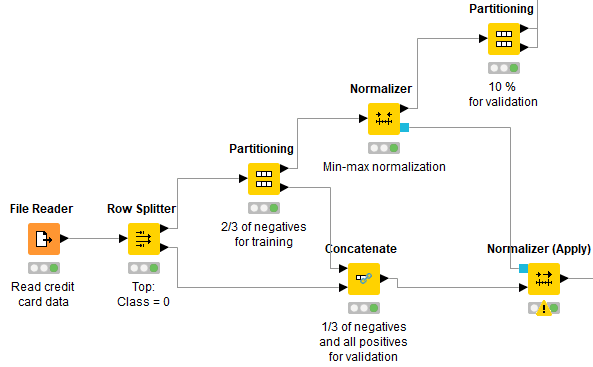
Figure 3: Preprocessing credit card data for fraud detection to feed a neural autoencoder. First we isolate all “normal” transactions from all fraudulent transactions; then we partition the “normal” transactions (⅔ -⅓ ): ⅔ move on to train and test the autoencoder, ⅓ is reunited with the fraudulent transactions and will form the validation set. Then all transaction data are normalized to fall into the [0,1] range, and finally, the data set with “normal” transactions only is split 90 percent (training) vs. 10 percent (test) to train and test the autoencoder.
Keras Deep Learning Extension
The Analytics Platform consists of a software core and a number of community-provided extensions and integrations. Such extensions and integrations greatly enrich the software core functionalities, tapping into, among others, the most advanced algorithms for artificial intelligence. This is the case, for example, of deep learning.
One of the Deep Learning extensions integrates functionalities from Keras libraries, which in turn integrate functionalities from TensorFlow within Python.
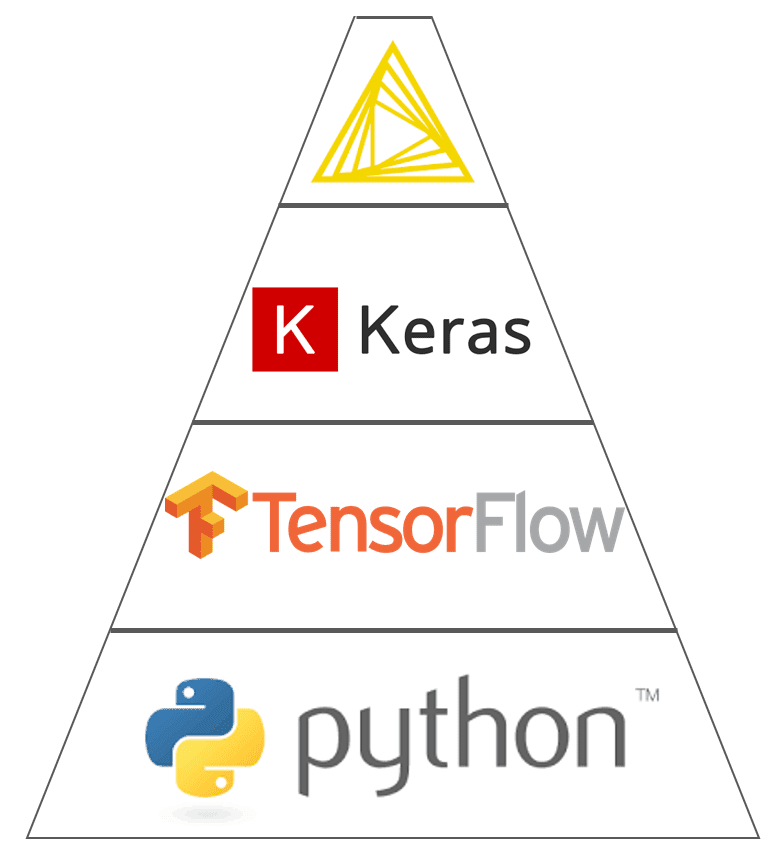
Figure 4. The Deep Learning Keras integration in Analytics Platform 3.7 encapsulates functions from Keras built on top of TensorFlow within Python.
In general, Deep Learning integrations bring deep learning capabilities to the Analytics Platform. These extensions allow users to read, create, edit, train and execute deep learning neural networks within the Analytics Platform.
In particular, Deep Learning Keras integration utilizes the Keras deep learning framework to read, write, create, train and execute deep learning networks. This Deep Learning Keras integration has adopted the GUI as much as possible. This means that a number of Keras library functions have been wrapped into nodes, most of them providing a visual dialog window to set the required parameters.
The advantage of using the Deep Learning Keras integration within the Analytics Platform is the drastic reduction of the amount of code to write, especially for preprocessing operations. Just by dragging and dropping a few nodes, you can build or import the desired neural architecture, which you can subsequently train with the Keras Network Learner node and apply with the DL Network Executor node — just a few nodes with easy configuration rather than calls to functions in Python code.
Installation
In order to make the Deep Learning Keras integration work, a few pieces of the puzzle need to be installed:
- Python (including TensorFlow)
- Keras
- Deep Learning Keras Extension
More information on how to install and connect all of these pieces can be found in the Deep learning – Keras Integration documentation page.
A useful video explaining how to install extensions can be found on this TV channel on YouTube.
Training and Testing the Autoencoder
The neural network (30-14-7-7-30) shown in Figure 1 is built absolutely codelessly using the nodes from the Deep Learning integration (Figure 5).
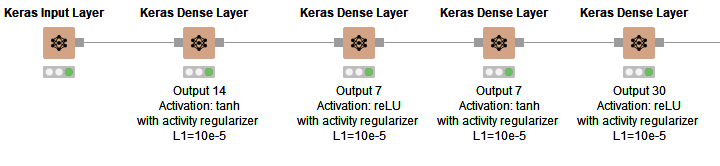
Figure 5: Structure of the neural network (30-14-7-7-30) trained to reproduce credit card transactions from the input layer onto the output layer.
- One input layer with as many dimensions (30) as the input features (Keras Input Layer node)
- A hidden layer that compresses the data into 14 dimensions using tanh activation function (Keras Dense Layer node)
- A hidden layer that compresses the data into 7 dimensions using reLU activation function (Keras Dense Layer node)
- One more hidden layer that transforms the input 7 dimensions into 7 other dimensions using tanh activation function (Keras Dense Layer node)
- One output layer that expands the data back to as many dimensions as in the input vector (30) using reLU activation function (Keras Dense Layer node)
This autoencoder is trained using the Keras Network Learner node, where the number of epochs and the batch size are set to 50, the training algorithm is set to Adam, and the loss function is set to be the mean squared error.

After training, the network is applied on the data from the test set to reproduce the input features using the DL Network Executor node, and it is saved for deployment as a Keras file using the Keras Network Writer node.
The next step would be to calculate the distance between the original feature vector and the reproduced feature vector and to define the optimal threshold K to discover fraud candidates.
The final workflow to train and test the neural autoencoder using credit card transaction data is shown in Figure 6. The workflow is downloadable for free from the EXAMPLES Server under: EXAMPLES/50_Applications/39_Fraud_Detection/Keras_Autoencoder_for_Fraud_Detection_Training.
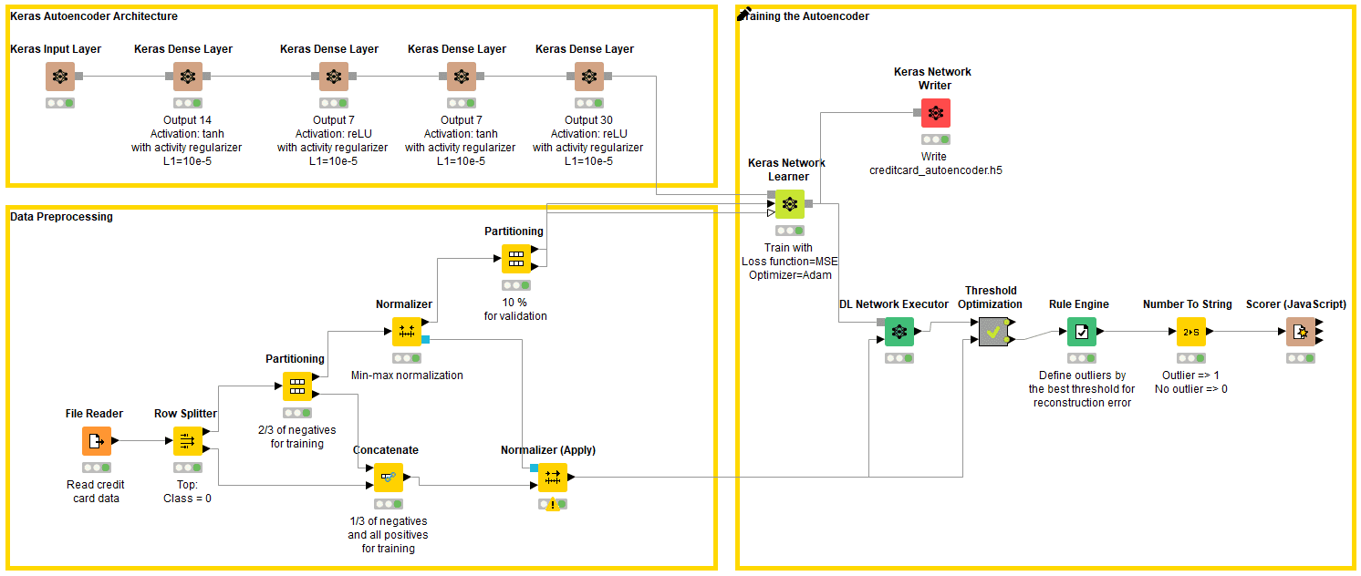
Figure 5: Workflow for training and testing a neural autoencoder for fraud detection on credit card transaction data. The workflow consists of the following steps: preprocessing the data, building the neural network architecture, training the network using a training set with only normal transactions, applying and testing the network, optimizing the value of threshold K against accuracy in the rule to detect fraud candidates, and finally saving the Keras model as the h5 file for deployment.
Optimizing Threshold K
The value of the loss function at the end of the autoencoder training though does not tell the whole story. It just tells how well the network is able to reproduce “normal” input data onto the output layer. To have a full picture of how well this approach performs in detecting anomalies, we need to apply the anomaly detection rule to the validation set. We will use the prediction accuracy on the validation set to optimize the value of threshold K.

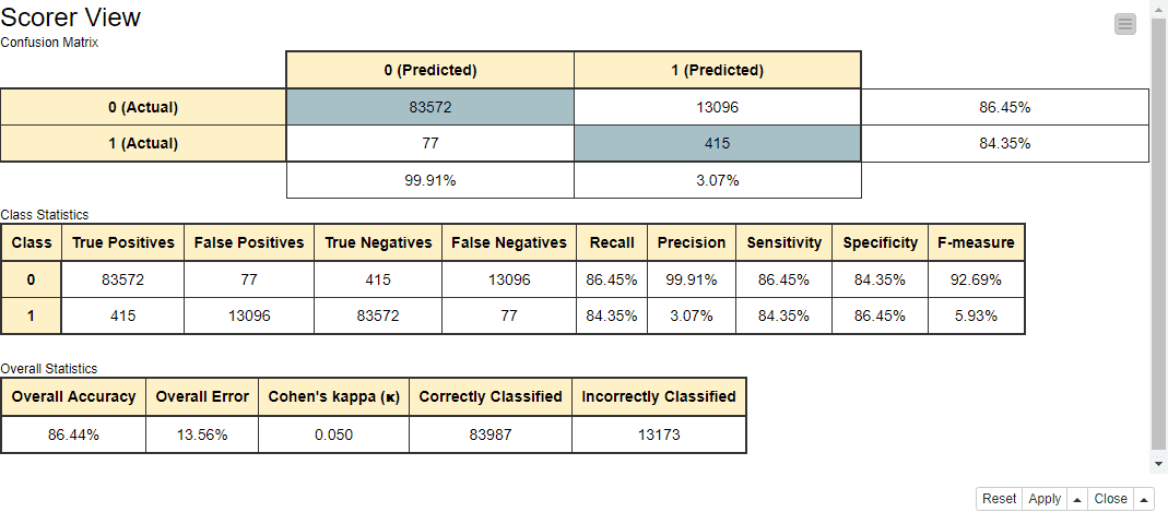
Figure 6: Performance metrics of the anomaly detection rule, based on the results of the autoencoder network for threshold K = 0.009.
As we can see in Figure 6, the autoencoder captures 84 percent of the fraudulent transactions and 86 percent of the legitimate transactions in the validation set. Considering the high imbalance between the number of normal and fraudulent transactions in the validation set (96,668 vs. 492), the results are promising.
Fraud Detector Deployment
Now that we are left with a network and a rule with acceptable performance, respectively, in reproducing the input data and in detecting anomalies, we need to implement the deployment workflow.
Like all deployment workflows, this workflow reads new transaction data, passes them through the model and anomaly detection rule, and finally predicts whether the current transaction is a fraud candidate or a legitimate transaction.
The deployment workflow is shown in Figure 7. It is downloadable for free from the EXAMPLES Server under EXAMPLES/50_Applications/39_Fraud_Detection/Keras_Autoencoder_for_Fraud_Detection_Deployment.
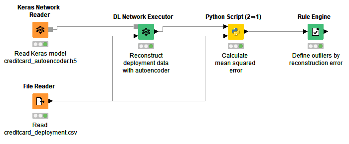
Figure 7: Deployment workflow for reading an autoencoder network stored in a Keras file and applying it to new transactions. In the Python Script node, reconstruction errors are calculated as mean squared errors between the original and reconstructed data. If the reconstruction error is greater than K=0.009, the transaction is considered as fraudulent. Otherwise, the transaction is considered as legitimate.
In this workflow, first the autoencoder model is read from the previously saved Keras file, using the Keras Network Reader node.
At the same time, data from new credit card transactions are read from file using the File Reader node. This particular file contains two new transactions with already normalized features.
Transaction data are fed into the autoencoder network and reproduced on the output layer with the DL Network Executor node.
Afterwards, the mean squared error between the original features and the reconstructed features is calculated using the Python Script (2 ⇒ 1) node with the following script:

The table below shows the reconstruction errors that the model produces for the two transactions:
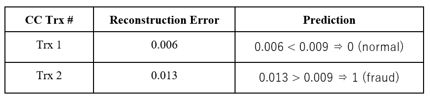
Table 1: Reconstruction errors and fraud class assignment for credit card transactions in the data set used for deployment.
As you can see, the system (autoencoder model + distance rule) defines the first transaction as normal and the second transaction as fraud.
Conclusions
The neural autoencoder offers a great opportunity to build a fraud detector even in the absence (or with very few examples) of fraudulent transactions. The idea stems from the more general field of anomaly detection and also works very well for fraud detection.
A neural autoencoder with more or less complex architecture is trained to reproduce the input vector onto the output layer using only “normal” data — in our case, only legitimate transactions. Thus, the autoencoder will learn to satisfactorily reproduce “normal” data. So, what about the anomalies?
For the anomalies, the reconstruction of the input vector by the autoencoder will hopefully fail. Therefore, if we calculate a distance (we used a mean square distance) between the original data vector and the reconstructed data vector, a much larger distance value will show up in the case of anomalies than in the case of “normal” data. That is, we can recognize candidates for fraudulent transactions from the value of the distance between the input vector and the reconstructed output vector. Translating this into a rule, if the distance value is beyond a threshold K, then we have a fraud/anomaly candidate.
The tricky part of this process is to define the threshold K. If we have no anomaly examples in our data set, we can use a high percentile of the data distribution. If we have at least some anomaly examples in our data set (as in our case study here), we can build a validation set and optimize the value of threshold K on it. We have followed this second approach.
All in all, the training of the network and the definition of threshold K was a relatively easy and fast process, reaching 84 percent of correct classification for fraudulent transactions and 86 percent of correct classification for “normal” transactions. However, as usual, more work could be done to improve performances. For example, the network parameters could be optimized, including experimentation with different activation functions and regularization parameters, a higher number of hidden layers and units per hidden layer, etc.
The whole process could also be forced to lean more toward frauds by introducing an expertise-based bias in the definition of threshold K. Sometimes, in fact, it might be preferable to tolerate a higher number of checkups on false positives than to miss even one fraudulent transaction!