Click to learn more about author Steve Miller.
A recent article in Atlantic highlights what had been emerging locally for over a year: Chicago suffered a disturbingly sharp spike in homicides in 2016, after a smaller but still noticeable surge in 2015. This at a time when other large cities like New York and Los Angeles were seeing lows in homicide and violent crime. The new president weighed in.
Several years ago, the City of Chicago committed to making its data accessible, establishing a portal. Early in 2016, I canvassed the site, looking for crime data — and found it. The data, covering reported crime starting in 2001, are sourced from the portal. A supplemental city community area spreadsheet is available at Chicago Metropolitan Agency for Planning.
For the analyses below, the 6.2M+ record crime csv file is loaded into an R data.table and subsequently wrangled using R packages dplyr, lubridate, and purrr. The community area spreadsheet is read into a data.table with readxl. The two data sources are then merged into the working data.table crimeplus.
Visualizations derive from R ggplot and plotly interactive graphics for the web. The R ggplotly package seamlessly connects ggplot and plotly, albeit not without discomfort. The graphs produced are accessible from a web browser in the links below.
The main drivers for the plots are frequencies computed with the crimeplus data.table. A flexible function, frequencisesdyn, allows the analyst to dynamically filter and dimensionalize frequency-producing queries.
The first look at the data focuses on homicide and violent crime in Chicago from 2001-2016 — or through January 2017, depending on the filter.
Alas, our homicide findings indeed confirm what’s been detailed in the news. The declining violent crime figures, though, offer hope, despite a 7.5% rise in 2016.
The remainder of the workbook details the R code to load and munge the data, produce frequencies, and graph the results.

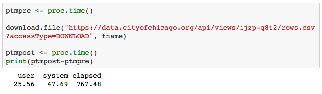
Download the Chicago crime “transaction” csv file. The data’s a week in arrears.
Download a spreadsheet housing data from Chicago’s 77 communities. Load the spreadsheet into an R data.table.

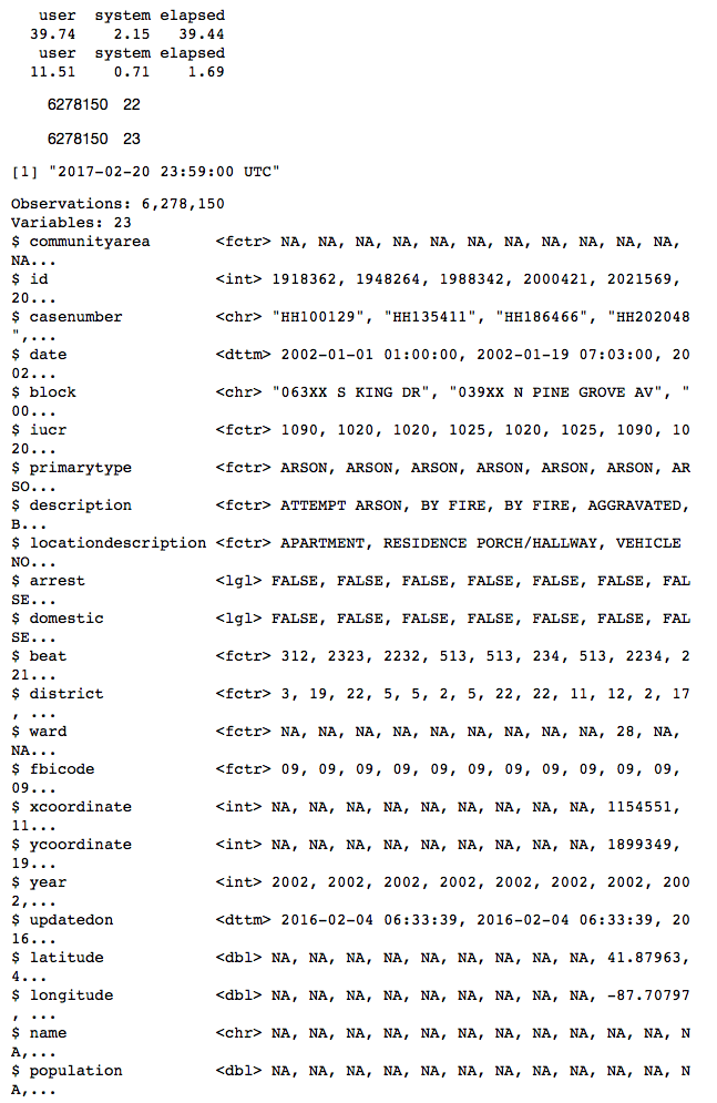
Read the downloaded crime transaction file into an R data.table.

Merge the communities and crime transaction data.tables into crimeplus. Tweak the logical, factor, and date variables. The 6,277,445 final records cover the period Jan 1, 2001 to Feb 20, 2017.

Define a dynamic frequencies function. Set filter variables and exercise frequenciesdyn on the crimeplus data.table. The counts are returned very fast.


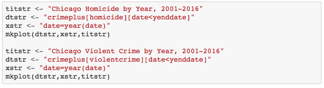
Logon to the plotly cloud. Define a ggplot/plotly function to display first homicide, then violent crime by year, by month, by hour of day, and finally by day of week. In addition to the data points and lines, each plot shows the overall mean frequency via a horizonal line, and traces a smoother to summarize direction. mkplot invokes frequenciesdyn to compute counts that feed the ggplot procedure.

Homicide and Violent Crime by Year.
Sadly, the homicide plot confirms the recent increases highlighted by a disturbing 2016. Hopefully, Chicago will experience a regression to the recent mean in coming years. But thankfully, the direction of overall violent crime is much more sanguine, down over 40% in 15 years. Maybe there is hope!
Homicide and Violent Crime by Month of Year.
Warm months are much more conducive to violent crime than cold ones.

Homicide and Violent Crime by Hour of Day.
Homicide is more common at night, while overall violent crime starts spiking in the afternoon.

Homicide and Violent Crime by Day of Week.
Not surprisingly, both homicide and violent crime peak on weekends.

Define a ggplot/plotly function to display first homicide, then violent crime by year — faceted by month. In addition to the data points and lines, each plot shows the overall mean frequency via a horizonal line, and traces a smoother to summarize direction. The mean frequency for each month is indicated by a dashed line.
The facet plots confirm and consolidate earlier observations, showing the sad uptick in homicide, along with the more hopeful overall decline in violent crime. The faceted monthly averages are telling, highlighting the seasonality in crime.
