Click to learn more about co-author Maarit Widmann.

Click to learn more about co-author Alfredo Roccato.

This is the second part of a the From Modeling to Scoring Series, see Part One here.

Wheeling like a hamster in the Data Science cycle? Don’t know when to stop training your model?

Model evaluation is an important part of a Data Science project, and it’s exactly this part that quantifies how good your model is, how much it has improved from the previous version, how much better it is than your colleague’s model, and how much room for improvement there still is.

In this series of blog posts, we review different scoring metrics: for classification, numeric prediction, unbalanced datasets, and other similar, more or less challenging model evaluation problems.

Today: Classification on Imbalanced Datasets

It is not unusual in machine learning applications to deal with imbalanced datasets such as fraud detection, computer network intrusion, medical diagnostics, and many more.

Data imbalance refers to unequal distribution of classes within a dataset, namely that there are far fewer events in one class in comparison to the others. If, for example, we have a credit card fraud detection dataset, most of the transactions are not fraudulent, and very few can be classed as fraud detections. This underrepresented class is called the minority class, and by convention, the positive class.

It is recognized that classifiers work well when each class is fairly represented in the training data.

Therefore, if the data is imbalanced, the performance of most standard learning algorithms will be compromised because their purpose is to maximize the overall accuracy. For a dataset with 99 percent negative events and 1 percent positive events, a model could be 99 percent accurate, predicting all instances as negative, though, being useless. Put in terms of our credit card fraud detection dataset, this would mean that the model would tend to classify fraudulent transactions as legitimate transactions. Not good!

As a result, overall accuracy is not enough to assess the performance of models trained on imbalanced data. Other statistics, such as Cohen’s kappa and F-measure, should be considered. F-measure captures both the precision and recall, while Cohen’s kappa takes into account the a priori distribution of the target classes.

The ideal classifier should provide high accuracy over the minority class, without compromising on the accuracy for the majority class.

Resampling to Balance Datasets

To work around the problem of class imbalance, the rows in the training data are resampled. The basic concept here is to alter the proportions of the classes (a priori distribution) of the training data in order to obtain a classifier that can effectively predict the minority class (the actual fraudulent transactions).

Resampling Techniques

• Undersampling: A random sample of events from the majority class is drawn and removed from the training data. A drawback of this technique is that it loses information and potentially discards useful and important data for the learning process.
• Oversampling: Exact copies of events representing the minority class are replicated in the training dataset. However, multiple instances of certain rows can make the classifier too specific, causing overfitting issues.
• SMOTE (Synthetic Minority Oversampling Technique): “Synthetic” rows are generated and added to the minority class. The artificial records are generated based on the similarity of the minority class events in the feature space.

Correcting Predicted Class Probabilities

Let’s assume that we train a model on a resampled dataset. The resampling has changed the class distribution of the data from imbalanced to balanced. Now, if we apply the model to the test data and obtain predicted class probabilities, they won’t reflect those of the original data. This is because the model is trained on training data that is not representative of the original data, and thus the results do not generalize into the original or any unseen data. This means that we can use the model for prediction, but the class probabilities are not realistic: We can say whether a transaction is more probably fraudulent or legitimate, but we cannot say how probably it belongs to one of these classes. Sometimes we want to change the classification threshold because we want to take more/fewer risks, and then the model with the corrected class probabilities that haven’t been corrected wouldn’t work anymore. 

After resampling, we have now trained a model on balanced data, i.e., data that contains an equal number of fraudulent and legitimate transactions, which is luckily not a realistic scenario for any credit card provider and, therefore — without correcting the predicted class probabilities — would not be informative about the risk of the transactions in the next weeks and months.

If the final goal of the analysis is not only to classify based on the highest predicted class probability but also to get the correct class probabilities for each event, we need to apply a transformation to the obtained results. If we don’t apply the transformation to our model, grocery shopping with a credit card in a supermarket might raise too much interest! 

The following formula shows how to correct the predicted class probabilities for a binary classifier [1]:

For example, if the proportion of the positive class in the original dataset is 1 percent and, after resampling, it is 50 percent, and the predicted positive class probability is 0.95, applying the correction it gives:

Example: Fraud Detection

When we apply a classification model to detect fraudulent transactions, the model has to work reliably on imbalanced data. Although few in number, fraudulent transactions can have remarkable consequences. Therefore, it’s worth checking how much we can improve the performance of the model and its usability in practice by resampling the data and correcting the predicted class probabilities. 

Evaluating the Cost of a Classification Model

In the real world, the performance of a classifier is usually assessed in terms of cost-benefit analysis: Correct class predictions bring profit, whereas incorrect class predictions bring cost. In this case, fraudulent transactions predicted as legitimate cost the amount of fraud, and transactions predicted as fraudulent — correctly or incorrectly — bring administrative costs. 

Administrative costs (Adm) are the expected costs of contacting the cardholder and replacing the card if the transaction was correctly predicted as fraudulent or reactivating it if the transaction was legitimate. Here we assume, for simplicity, that the administrative costs for both cases are identical.

The cost matrix below summarizes the costs assigned to the different classification results. The minority class, “fraudulent,” is defined as the positive class, and “legitimate” is defined as the negative class.

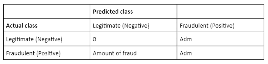
Based on this cost matrix, the total cost of the model is:

Finally, the cost of the model will be compared to the amount of fraud. Cost reduction tells how much cost the classification model brings compared to the situation where we don’t use any model:

The Workflow

In this example, we use the “Credit Card Fraud Detection” dataset provided by Worldline and the Machine Learning Group of ULB (Université Libre de Bruxelles) on big data mining and fraud detection. The dataset contains 284,807 transactions made by European credit card holders during two days in September 2013. The dataset is highly imbalanced: 0.172 percent (492 transactions) were fraudulent, and the rest were normal. Other information on the transactions has been transformed into principal components.

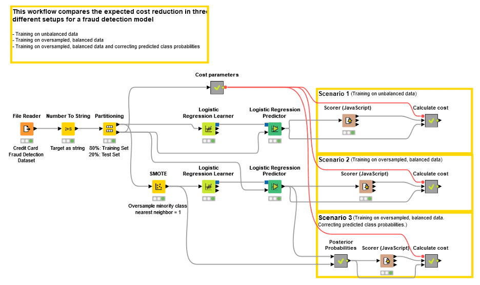
The workflow in Figure 1 shows the overall process of reading the data, partitioning the data into a training and test set, resampling the data, training a classification model, predicting and correcting the class probabilities, and evaluating the cost reduction. We selected SMOTE as the resampling technique and logistic regression as the classification model. Here we estimate administrative costs to be 5 euros.

The workflow provides three different scenarios for the same data: 

1. Training and applying the model using imbalanced data

2. Training the model on balanced data and applying the model to imbalanced data without correcting the predicted class probabilities

3. Training the model on balanced data and applying the model to imbalanced data where the predicted class probabilities have been corrected

Estimating the Cost for Scenario 1 Without Resampling

A logistic regression model provides these results:

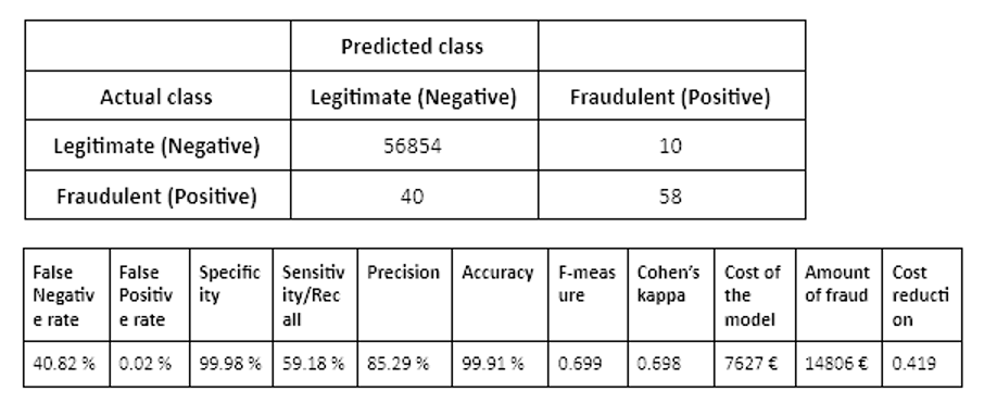
The setup in this scenario provides good values for F-measure and Cohen’s kappa statistics, but a relatively high False Negative Rate (40.82 percent). This means that more than 40 percent of the fraudulent transactions were not detected by the model — increasing the amount of fraud and, therefore, the cost of the model. The cost reduction of the model compared to not using any model is 42 percent.

Estimating the Cost for Scenario 2 with Resampling

A logistic regression model trained on a balanced training set (oversampled using SMOTE) yields these results:

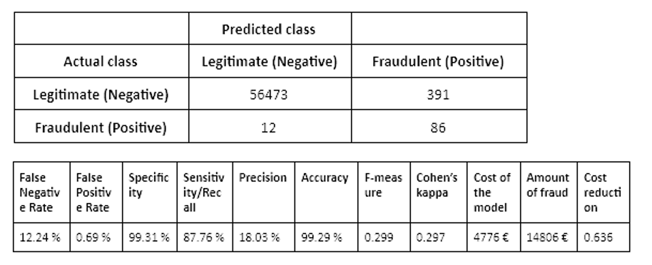
The False Negative Rate is very low (12.24 percent), which means that almost 90 percent of the fraudulent transactions were detected by the model. However, there are a lot of “false alarms” (391 legitimate transactions predicted as fraud) that increase administrative costs. However, the cost reduction achieved by training the model on a balanced dataset is 64 percent — higher than what we could reach without resampling the training data. The same test set was used for both scenarios.

Estimating the Cost for Scenario 3 with Resampling and Correcting the Predicted Class Probabilities

A logistic regression model trained on a balanced training set (oversampled using SMOTE) yields these results when the predicted probabilities have been corrected according to the a priori class distribution of the data:

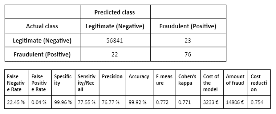
As the results for this scenario in Table 4 show, correcting the predicted class probabilities leads to the best model of these three scenarios in terms of the greatest cost reduction. 

In this scenario, where we train a classification model on oversampled data and correct the predicted class probabilities according to the a priori class distribution in the data, we reach a cost reduction of 75 percent compared to not using any model. 

Of course, the cost reduction depends on the value of the administrative costs. Indeed, we tried this by changing the estimated administrative costs and found out that this last scenario can attain cost reduction as long as the administrative costs are 0.80 euros or more.

Summary

Often, when we train and apply a classification model, the interesting events in the data belong to the minority class and are therefore more difficult to find: fraudulent transactions among the masses of transactions, disease carriers among the healthy people, and so on.

From the point of view of the performance of a classification algorithm, it’s recommended to make the training data balanced. We can do this by resampling the training data. Now, the training of the model works better, but how about applying it to new data, which we suppose to be imbalanced? This setup leads to biased values for the predicted class probabilities because the training set does not represent the test set or any new, unseen data. 

Therefore, to obtain optimal performance of a classification model together with reliable classification results, correcting the predicted class probabilities by the information on the a priori class distribution is recommended. As the use case in this blog post shows, this correction leads to better model performance and concrete profit.

References

1.Marco Saerens, Patrice Latinne, and Christine Decaestecker. Adjusting the outputs of a classifier to new a priori probabilities: a simple procedure. Neural computation 14(1):21–41, 2002.