
Click to learn more about author Maarit Widmann.
In the “Will They Blend?” blog series, we experiment with the most interesting blends of data and tools.
Whether it’s mixing traditional sources with modern data lakes, open-source devops on the cloud with protected internal legacy tools, SQL with noSQL, web-wisdom-of-the-crowd with in-house handwritten notes, or IoT sensor data with idle chatting, we’re curious to find out: Will they blend? Want to find out what happens when IBM Watson meets Google News, Hadoop Hive meets Excel, R meets Python, or MS Word meets MongoDB?
Read the previous blog in the series here.
Today’s challenge: Blend data on a SAP system that is accessed in two ways
1. The legacy way – via the JDBC driver of the database, SAP HANA, for example, and
2. The new way – via the Theobald Xtract Universal Server
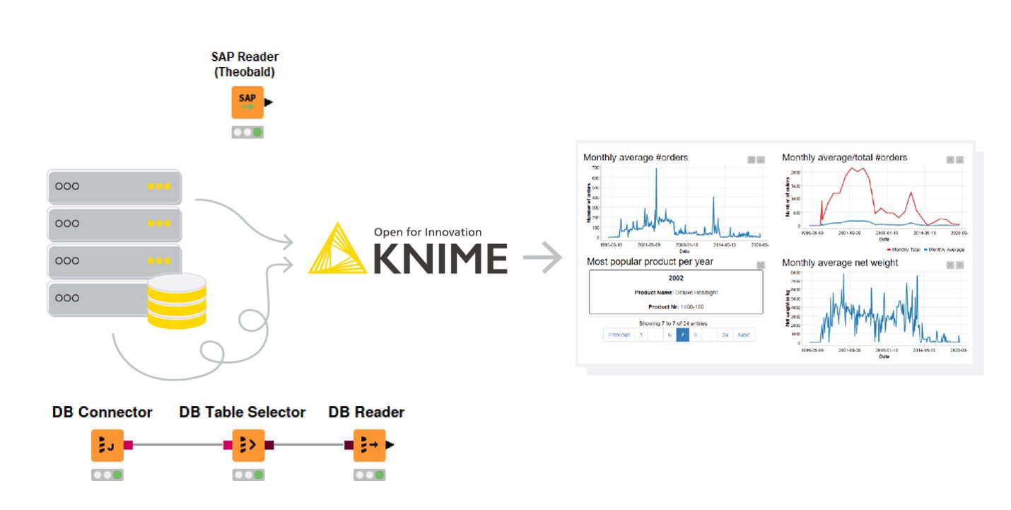
The legacy way requires a few steps: registering the JDBC driver of the SAP HANA database in KNIME, connecting to the database with the DB Connector node, selecting a table on the connected database, and reading it into the database. Using the SAP integration available from the Analytics Platform version 4.2 forward, you can access and load SAP data just by one node called SAP Reader (Theobald).
In our example, we extract KPIs from orders data, and show their development over time. We access the data about the submitted orders the legacy way. The data about the features of the ordered items are available on the Theobald Xtract Universal Server, so we read this data with the SAP Reader (Theobald) node. We connect to both systems from within the platform, join the data on the sales document key column available in both tables, and show the historical development of a few KPIs in an interactive dashboard: Is the number of orders increasing over time? What is the most popular product per year? Let’s take a look!
Challenge: Access SAP data via Theobald and via the JDBC driver of the SAP HANA database
Topic: Calculate KPIs of orders/items data and visualize the historical development of the KPIs in an interactive dashboard
Access Mode: Connect to Theobald Xtract Universal Server and to SAP HANA database
Integrated Tools: SAP, Theobald
The Experiment
The workflow in Figure 2 shows the steps in accessing the SAP data via Theobald (top branch) and via the JDBC driver of the database (bottom branch). The data for this experiment is stored in the Sales Document: Item Data and Sales Document: Header Data tables included in SAP ERP. After accessing the data, we join the tables, and extract year and month from the timestamps in order to calculate the KPIs at a meaningful granularity. Next, we calculate four different KPIs: total number of orders per month, average number of orders per month, average net weight of an order in each month, and the most popular product in each year. The KPIs are shown in the interactive view of the KPI Dashboard component (Figure 3).
- Download the workflow Will They Blend: SAP Theobald meets SAP HANA from the Hub.
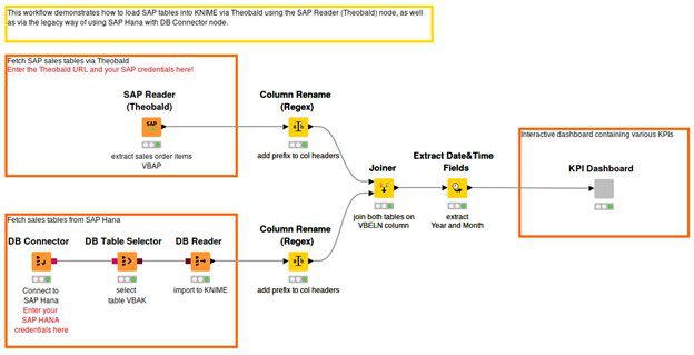
Figure 2: A workflow to access SAP data via Theobald and via the JDBC driver of the SAP HANA database, and to blend and preprocess data before calculating and visualizing KPIs in an interactive dashboard.
Accessing Theobald Xtract Universal Server
We want to access the “Sales Document: Item Data” table that contains detailed information about item orders (each row contains details of a specific item of an order) and is accessible via the Theobald Xtract Universal Server. The server provides a so-called table extraction feature where we can extract specific tables/views from various SAP systems and store them as “table extraction” queries. The SAP Reader (Theobald) node is able to connect to the given Xtract Universal Server to execute those queries and import the resulting data.
1. Open the configuration dialog of the node, and enter the URL to the Theobald Xtract Universal Server. Click the Fetch queries button to fetch all available extraction queries on the server. We can then select one query from the drop-down list. In our case it is the “Sales Document: Item Data” table. Note that it is necessary to provide SAP credentials in the authentication section if the selected query is connected to a protected SAP system.
2. Executing the node will execute the selected query on the Xtract Universal server and imports the data into a table.
Accessing SAP HANA
We want to access the “Sales Document: Header Data” table that contains information about the submitted orders and is available on the SAP HANA database on a locally running server. We can access the database, like any other JDBC-compliant database that doesn’t have a dedicated connector node, with the DB Connector node. In the configuration dialog of the DB Connector node, we can select the JDBC driver of an arbitrary database in the Driver Name field. In order to make our preferred database SAP HANA show in the Driver Name menu, we need to register its JDBC driver first.
- To register a JDBC driver, go to File → Preferences → KNIME → Database. The driver (.jar file) is installed as part of the SAP HANA client installation. To find where the JDBC driver is located, please check the SAP HANA documentation. Then we can add it to KNIME by following the steps described here in the Database Extension Guide.
- After registering the JDBC driver, open again the configuration dialog of the DB Connector node, select the newly registered JDBC driver in the menu, for example, sap: [ID: sap_id], and specify the database URL, for example, jdbc:sap://localhost:39015. Also provide the credentials with one of the authentication methods.
- The connection to the SAP HANA database is now created. Continue with the DB Table Selector node to select a table on the database and the DB Reader node to read the data into a table.
Blending Data and Calculating the KPIs
After accessing the two tables, we join them on the sales document key (VBELN column), and get a table that contains information on both the submitted orders and the items included in each order. Since the current granularity of the data is daily, and the time range of the data reaches from January 1997 to May 2020, we aggregate the data at a monthly level before calculating the KPIs.
Results
The interactive view output of the KPI Dashboard component (Figure 3) visualizes the KPIs. In the line plot in the top left corner we can see that the average number of orders per month was the highest at the beginning of 2000, and since 2014 it stagnates at a relatively low level. Yet in the past there were some quieter periods followed by periods with more orders, for example, the low around 2008 followed by a peak around 2013. We can find a similar kind of pattern in the line plot in the top right corner that shows in addition the total number of orders per month.
In the tile view in the bottom left corner, we can browse through the most popular products for each year. And finally, in the line plot in the bottom right corner, we can see that the ordered items have become lighter over time, or the orders contain fewer items than before and have therefore less weight. An especially remarkable decrease in the average weight of an order happened around 2014.
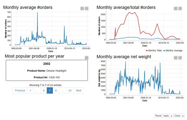
Figure 3: Interactive dashboard visualizing the KPIs that were calculated after accessing and blending the orders/items data available as SAP tables.
Do They or Don’t They?
In the dashboard shown in Figure 3, the product names and weights come from the “Sales Document: Item Data” table, accessed via Theobald Xtract Universal Server, whereas the order counts come from the “Sales Document: Header Data” table, accessed via the JDBC driver of a SAP HANA database.
All this information can be visualized in one dashboard, so yes, they blend!