Click to learn more about author Rosaria Silipo.

The co-authors of this column were Kathrin Melcher and Simon Schmid

Automatic machine translation has been a popular subject for machine learning algorithms. After all, if machines can detect topics and understand texts, translation should be just the next step.

Machine translation can be seen as a variation of natural language generation. In a previous project, we worked on the automatic generation of fairy tales (see “Once upon a Time … by LSTM Network”). Here a recurrent neural network (RNN) with a long short-term memory (LSTM) layer was trained to generate sequences of characters on texts from the Grimm’s fairy tales. The result was a new text in a Grimm’s fairy tale style.

Today, we extend this example of language generation to language translation. In particular, we try to address the need to make communication between the German and U.S. offices easier by attempting an English to German translation experiment.

A dataset suitable for this task is available and downloadable for free at: www.manythings.org/anki/. This dataset contains a number of sentences in both languages commonly used in everyday life. It consists of two columns only: the original short text in English and the corresponding translation in German.

Figure 1. An excerpt from the English <-> German translation dataset.

As for language generation, machine translation can be implemented at word level or at character level. In the first case, the next word is predicted given the previous sequence of words. In the second case, the next character is predicted given the previous sequence of characters. Since we have accumulated some experience in text generation at character level, we will continue with machine translation at character level.

Again, as for language generation, an RNN with one (or more) LSTM layer(s) might prove suitable for the task. For this task, however, we are dealing with two languages. Thus, we adopt a slightly modified neural architecture with two LSTM layers: one for the original language text and one for the target language text. This architecture is known as the encoder-decoder RNN structure.

The Encoder-Decoder RNN Structure

The task of machine translation consists of reading text in one language and generating text in another language. When neural networks are used for this task, we talk about neural machine translation (NMT)[i] [ii].

Within NMT, the encoder-decoder structure is quite a popular RNN architecture. This architecture consists of two components: an encoder network that consumes the input text and a decoder network that generates the translated output text ⁱⁱ. The task of the encoder is to extract a fixed sized dense representation of the different length input texts. The task of the decoder is to generate the corresponding text in the destination language, based on the dense representation from the encoder (Fig. 2). Usually both networks are RNNs, often LSTMs.

Figure 2. The encoder-decoder neural architecture.

A common way of representing RNNs is to unroll them into a sequence of copies of the same static network A, each one fed by the hidden state of the previous copy h(t−1) and by the current input x(t). The unrolled RNN can then be trained with the Backpropagation Through Time (BPTT) algorithm [iii] (Fig. 3).

Let’s choose an LSTM layer for the encoder and decoder networks. An LSTM network is a particular type of RNN, relying on internal gates, to selectively remove (forget) or add (remember) information from/to the cell state C(t) based on the input values x(t) and the hidden state h(t−1) at each time step t (see “Once upon a Time … by LSTM Network” on the KNIME blogⁱ for more details on RNNs and LSTM layers).

Figure 3. LSTM networks are RNNs, which could be represented as a sequence of copies of static network A connected via their hidden states. Below is a representation of an LSTM network trained to generate free text.

Deep Learning Keras – Integration

The Deep Learning Keras Integration is an open source platform for Data Science, covering all your data needs from data ingestion and data blending to data visualization, from machine learning algorithms to data wrangling, from reporting to deployment, and more. It is based on a graphical user interface (GUI) for visual programming. This makes it very intuitive and easy to use, considerably reducing the learning time. Deep Learning Keras has been designed to be open to different data formats, data types, data sources, and data platforms as well as external tools, for example, Python and R.

Because of its graphical interface, computing units in the platform are small colorful blocks, named “nodes.” Assembling nodes in a pipeline, one after the other, implements a data processing application. The pipeline is called “workflow” (Figs. 6 and 7).

The platform consists of a software core and a number of community provided extensions and integrations. Such extensions and integrations greatly enrich the software core functionalities, tapping, among others, into the most advanced algorithms for Artificial Intelligence. This is the case, for example, with deep learning.

The Deep Learning extension integrates functionalities from the Keras libraries, which in turn integrate functionalities from TensorFlow in Python (Fig. 4).

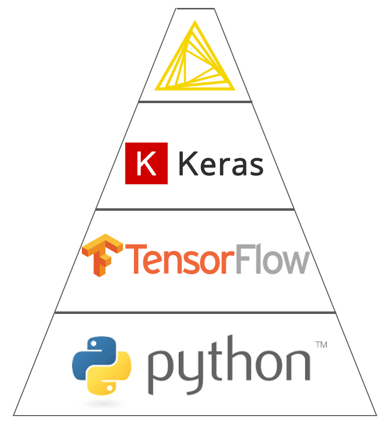
Figure 4. The deep learning integration 3.7 encapsulates functions from Keras built on top of TensorFlow in Python.

Figure 5. Some of the nodes available in the deep learning integration. Notice the DL4J integration and the Keras integration. Especially within the Keras integration, notice the many nodes available to build specific network layers. A number of nodes are also available to train networks in Keras, TensorFlow and Python.

The advantage of using the Keras Integration is the drastic reduction in the amount of code to write. Indeed, a number of Keras library functions have been wrapped into the nodes, most of them providing a visual dialog window and a few of them allowing the integration of additional Keras/TensorFlow libraries via Python code.

In Figure 5, you can see all of the nodes available in the Keras Integration. A large number of nodes implement neural layers: input and dropout layers in Core, LSTM layers in Recurrent, and Embedding layers in the Embedding sub-category. Then, of course, the Learner, Reader and Writer nodes to respectively train, retrieve and store a network.

Two important nodes are the DL Python Network Executor and DL Python Network Editor. These two nodes respectively allow custom execution and custom editing of a Python compatible Deep Learning network via Python script, including Jupyter notebook. These two nodes effectively bridge Keras nodes with all other not yet integrated Keras/TensorFlow library functions.

The Training Workflow

In theory, training should be performed using the predicted character from the previous step. In practice, however, it is possible to obtain better training performances using the so-called “teacher forcing” technique. Here, the actual previous character instead of the previous prediction is fed into the next network copy, which greatly benefits the training procedure (ⁱⁱⁱ p.372). This forced feeding of the actual characters must be removed in the deployment workflow.

Therefore, we need three different character sequences to train the network:

1. The input sequence into the encoder. That is the index-encoded input character sequence for the original language.
2. The input sequence into the decoder. That is the index-encoded character sequence for the translation language.
3. The target sequence, which is the input sequence to the decoder shifted by one step.

Remember that a network doesn’t understand characters but only numerical values. The character input sequences need to be transformed into numerical input sequences via one of the many text encoding strategies available.

The training workflow in Figure 6 covers all the required steps:

• English and German text preprocessing
• Network structure definition for the encoder and the decoder
• Network training
• Network structure modification for both encoder and decoder via Python editing
• Model deployment and evaluation

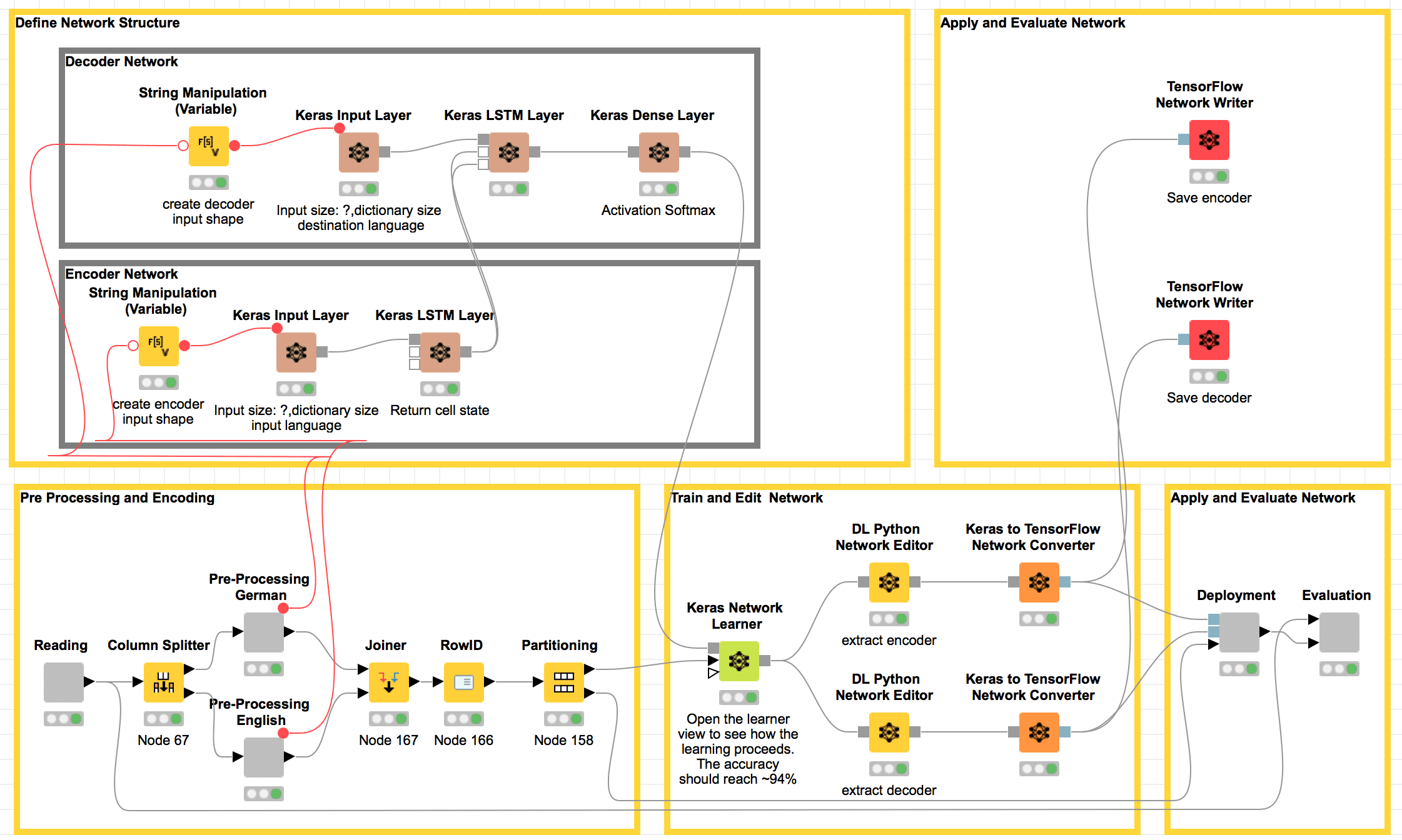
Figure 6. Workflow to build, train and evaluate a neural network for automatic translation from English to German. In the top left frame, the brown nodes each add one layer to the neural network for the training phase: an input layer and an LSTM layer for the English (encoder) and German (decoder) text, respectively, and one dense layer to produce character probabilities at the end. The frame under the network construction nodes transforms the English and German texts into index-based encoding sequences. Still in the lower part, nodes in the central frame train the whole network and then split it into encoder and decoder via DL Python Network Editor nodes. Finally, Deployment and Evaluation nodes apply the network to the test set and evaluate the translation results.

Network Structure Definition

The upper part of the workflow, including the brown nodes, defines the neural network structure. The brown nodes each build one type of layer in the neural network.

The encoder network is made of two layers:

1. An input layer implemented via the Keras Input Layer node. This layer accepts input tensors of integer indexes, with variable sequence length and same size as the character dictionary size of the input language (English). In our example, the input tensor for English has size [?, dictionary size input language], i.e., [?,70].

• An LSTM Layer via a Keras LSTM Layer node: In this node, the checkbox “return state” must be enabled to pass the hidden states to the upcoming decoder network.

The decoder network is made of three layers:

1. An input layer via a Keras Input Layer node. This layer defines the shape of the input tensor, with variable sequence length and same size as the character dictionary size of the input language (German). In our example, the input tensor for German has size [?, dictionary size destination language], i.e., [?, 85].

• An LSTM layer via a Keras LSTM Layer node. This layer has two inputs: the character sequence for the text in the destination language and the hidden states from the encoder LSTM layer. In its configuration window, the checkboxes “return sequence” and “return state” are both enabled to return the hidden state as well as the next character prediction.

• Last, a dense layer via a Keras Dense Layer node to produce the probability vector for all dictionary characters. In the configuration window, the activation function softmax is selected to have 85 units, i.e., the size of the dictionary of the destination language.

Text Preprocessing and Encoding

In the lower left corner of the workflow, we find the nodes dedicated to text preprocessing and encoding. Remember that we have two texts to preprocess and encode: one in English and one in German. We use index-based encoding for both of them.

In addition, all input sequences need a Start Token, set to 1, to mark the beginning of the character sequence. All target sequences need an End Token, set to 0, at the end, to mark the end of the character sequence. In addition, since all character sequences must have the same length as defined by the corresponding input layer, zero-padding and truncation are also applied where needed. All of these operations are implemented in the gray nodes named “Preprocessing German” and “Preprocessing English” for German and English, respectively.

These same encoding and preprocessing steps are described in detail in the “Once Upon A Time …  by LSTM Network” blog postⁱ.

Network Training and Editing

In the middle lower part of the workflow in Figure 6, the network is trained with the BPTT algorithm by executing the Keras Network Learner node.

Note that the output of the dense softmax layer gives the probability distribution for all index-encoded characters of the German language. The predicted character can be selected as the one with the highest probability or via an additional lambda layer.

After the network has been trained, it needs a bit of a post-processing before deployment, such as:

• Separate the encoder and decoder part of the network.
• Introduce a lambda layer with an argmax function to select one of the characters with the highest probability in the softmax layer. The lambda layer adds noise into the selection process, which then leads to a less deterministic character selection.

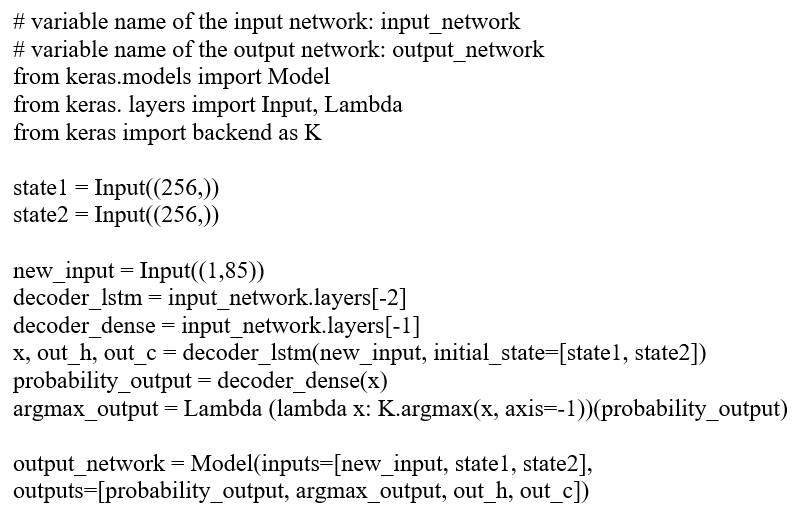
The DL Python Network Editor nodes allow those changes to be made to the network structure with a relatively simple Python code snippet. The Python code to extract the decoder network and to introduce the lambda layer is:

For faster deployment execution, the encoder and decoder Keras networks are converted to TensorFlow and saved separately.

The Deployment Workflow

In the deployment workflow (Fig. 7), English sentences have to pass through the encoder and the decoder networks in two subsequent steps. Two TensorFlow Network Reader nodes read respectively the encoder and the decoder network.

Two DL Network Executor nodes feed the two networks with the input data table of English sentences. The first DL Network Executor node presents an English character to the encoder and produces the corresponding hidden state. The second DL Network Executor node presents this hidden state from the encoder to the decoder network to produce the predicted index-encoded character for the German sentence.

Figure 7. The deployment workflow applies the encoder and decoder network to a new English sentence. Notice that the encoder and decoder networks are retrieved from two separate TensorFlow files.

Finally, the German dictionary is applied to extract the character from index-based encoding to get the final translated sentence. Below is an excerpt of the translation results.

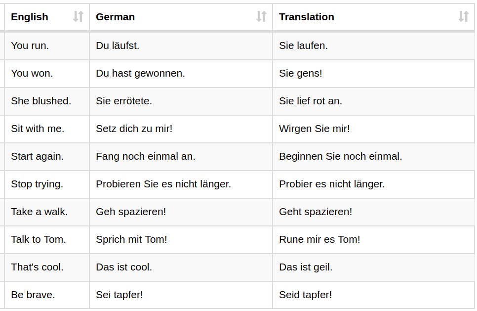
Figure 8. Final results of the deployed translation network on new sentences. “English” is the input sentence, “German” is the proposed target, and “Translation” is the actual German text produced by the network.

Conclusion

We’ve explored the topic of neural machine translation, specifically on a translation task from English to German. In order to solve this problem, we dove into the Deep Learning Keras Integration, and we implemented an almost codeless deep learning workflow via the GUI.

The neural network architecture consisted of a classic encoder-decoder structure operating at the character level. The encoder network was trained to represent the English character sequence as a numerical intermediate set of features. The decoder network consumed this intermediate set of numerical features and transformed them into the final sequence of characters for the translation.

Both networks were built codelessly by using the nodes from the Keras Integration: one node for the input layer, one node for the LSTM layer, one node for the dense output layer.

The joint network, derived from the combination of encoder and decoder, was trained using a teacher forcing paradigm. At the end of the training phase and before deployment, a lambda layer was inserted in the decoder part to add a pinch of randomness to the character prediction process. This means that the trained network structure was modified at the end of the training process. In order to do that, a DL Python Network Editor node took care of splitting the decoder and the encoder networks and adding the lambda layer. This was the only part involving a short simple snippet of Python code.

Eventually, in deployment, the encoder accepts the character sequence of an English sentence and generates the sequence of temporary numerical features. Then, the decoder uses the previously predicted German character and the current set of temporary features from the encoder and generates the next predicted character for the German sentence.

Translation results are so far satisfactory but could still be improved with more dta, parameter optimization, and longer network training.

Cheers! Zum Wohl!

[i] Yonghui Wu, et al., “Google’s Neural Machine Translation System: Bridging the Gap between Human and Machine Translation,” arXiv:1609.08144v2 [cs.CL], Oct. 8, 2016

[ii] Prakhar Mishra, “A Concise Introduction to Neural Machine Translation,” https://hackernoon.com/a-concise-introduction-to-neural-machine-translation-d925ee1ff5df

[iii] Ian Goodfellow, Yoshua Bengio and Aaron Courville, “Deep Learning,” The MIT Press, 2016