Click to learn more about author Kathrin Melcher.

Regularization can be used to avoid overfitting. But what actually is regularization, what are the common techniques, and how do they differ?

Well, according to Ian Goodfellow [1]:

“Regularization is any modification we make to a learning algorithm that is intended to reduce its generalization error but not its training error.”

In other words: regularization can be used to train models that generalize better on unseen data, by preventing the algorithm from overfitting the training dataset.

So how can we modify the logistic regression algorithm to reduce the generalization error?

Common approaches I found are Gauss, Laplace, L1 and L2. The Analytics Platform supports Gauss and Laplace and indirectly L2 and L1.

Gauss or L2, Laplace or L1? Does it make a difference?

It can be proven that L2 and Gauss or L1 and Laplace regularization have an equivalent impact on the algorithm. There are two approaches to attain the regularization effect.

First Approach: Adding a Regularization Term

To calculate the regression coefficients of a logistic regression the negative of the Log Likelihood function, also called the objective function, is minimized:

You can check this YouTube video

But why should we penalize high coefficients? If a feature occurs only in one class it will be assigned a very high coefficient by the logistic regression algorithm [2]. In this case the model will learn all details about the training set, probably too perfectly.

The two common regularization terms, which are added to penalize high coefficients, are the l1 norm or the square of the norm l2 multiplied by ½, which motivates the names L1 and L2 regularization.

Note. The factor ½ is used in some derivations of the L2 regularization. This makes it easier to calculate the gradient, however it is only a constant value that can be compensated by the choice of the parameter λ.

i.e. the sum of the absolute values of the coefficients, aka the Manhattan distance.

The regularization term for the L2 regularization is defined as:

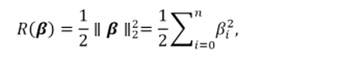
i.e. the sum of the squared of the coefficients, aka the square of the Euclidian distance, multiplied by ½.

Through the parameter λ we can control the impact of the regularization term. Higher values lead to smaller coefficients, but too high values for λ can lead to underfitting.

Second Approach: Bayesian View of Regularization

The second approach assumes a given prior probability density of the coefficients and uses the Maximum a Posteriori Estimate (MAP) approach [3]. For example, we assume the coefficients to be Gaussian distributed with mean 0 and variance σ² or Laplace distributed with variance σ².

In this case we can control the impact of the regularization through the choice of the variance. Smaller values lead to smaller coefficients. Here, however, small values of σ² can lead to underfitting.

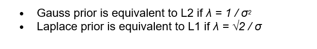
The two mentioned approaches are closely related and, with the correct choice of the control parameters λ and σ², lead to equivalent results for the algorithm. In KNIME the following relationship holds:

Is Regularization Really Necessary?

To understand this part, we designed a little experiment, where we used as subset of the Internet Advertisement dataset from the UCI Machine Learning Repository. The subset contains more input features (680) than samples (120), thus favoring overfitting.

The Workflow

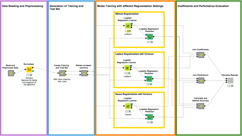
In the workflow in figure 1, we read the dataset and subsequently delete all rows with missing values, as the logistic regression algorithm is not able to handle missing values.

Next we z-normalize all the input features to get a better convergence for the stochastic average gradient descent algorithm.

Note. If you’re interested in interpreting the coefficients through the odds ratio, you should take into account the data normalization.

Then, we create a training and a test set and we delete all columns with constant value in the training set. At this point, we train three logistic regression models with different regularization options:

• Uniform prior, i.e. no regularization,
• Laplace prior with variance σ² = 0.1
• Gauss prior with variance σ² = 0.1.

Note. We used the default value for both variances. By using an optimization loop, however, we could select the optimal variance value.

Next, we join the logistic regression coefficient sets, the prediction values and the accuracies, and visualize the results in a single view.

Figure 1. In this workflow we first read the advertisement dataset, normalize the input features, create a training subset with 120 samples and 680 features, and train three logistic regression models with different prior settings. In the last step we join and visualize the results.

Impact on performance

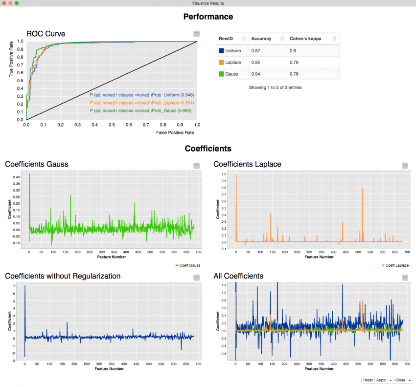
In figure 2 the results are displayed. First, let’s consider only the upper part, which shows different performance measures for the three models, e.g. the accuracies, Cohen’s Kappa and the ROC curve.

In general we can say that for the considered example, with a dataset favoring overfitting, the regularized models perform much better.

For example the accuracy increases from 87.2% to 93.9% for Gauss and to 94.8% for Laplace. We also get higher values for Cohen’s Kappa and for the area under the curve.

Gauss or Laplace: What is the impact on the coefficients?

So far we have seen that Gauss and Laplace regularization lead to a comparable improvement on performance. But do they produce also similar models?

It’s when we consider the coefficients that we discover some differences. In the lower part of the interactive view in figure 2 the values of the coefficients over the feature numbers are displayed for the different priors. Notice that the plots have different ranges on the y axis!

The two upper plots show the coefficients for Laplace and Gauss prior. They clearly show that the coefficients are different!

The most striking result is observed with Laplace prior, where many of the coefficients end up to be zero. Indeed, it is said that Laplace regularization leads to sparse coefficient vectors and logistic regression with Laplace prior includes feature selection [2][3].

In the case of Gauss prior we don’t get sparse coefficients, but smaller coefficients than without regularization. In other words, Gauss leads to smaller values in general, while Laplace leads to sparse coefficient vectors with a few higher values.

The two lower line plots show the coefficients of logistic regression without regularization and all coefficients in comparison with each other. The plots show that regularization leads to smaller coefficient values, as we would expect, bearing in mind that regularization penalizes high coefficients.

Figure 2. This is the view from the last wrapped metanode from the workflow reported in figure 1. The upper part of the view shows the performance measures for the different priors. We see that all three performance measures increase if regularization is used. In the lower part the coefficients for the different priors are plotted over the feature numbers. The plots show the different impact of Gauss and Laplace prior on the coefficients and that regularization in general leads to smaller coefficients.

Summary

In conclusion we can say that:

• L2 and Gauss regularizations are equivalent. The same for L1 and Laplace.
• Regularization can lead to better model performance
• Different prior options impact the coefficients differently. Where Gauss generally leads to smaller coefficients, Laplace results in sparse coefficient vectors with just a few higher value coefficients.

References

[1] Ian Goodfellow, Yushua Bengio, Aaron Courville, “Deep Learning”, London: The MIT Press, 2017.

[2] Daniel Jurafsky, James H. Martin, “Logisitic Regression“, in Speech and Language Processing.

[3] Andrew Ng, “Feature selection, L1 vs L2 regularization, and rotational invariance”, in: ICML ’04 Proceedings of the twenty-first international conference on Machine learning, Stanford, 2004.

[4] Bob Carpenter, “Lazy Sparse Stochastic Gradient Descent for Regularized Multinomial Logistic Regression”, 2017.