Click to learn more about author Thomas Frisendal.

One of the major contributions of Dr. Ted Codd’s relational model is the focus on the importance of functional dependencies. In fact, normalization is driven by a modeler’s desire for a relation where strict functional dependency applies across all the binary relations between the designated primary key and the fields depending on it. It is a quality assurance thing, really. This way functional dependencies are very important contributors to the structural description of the information being modeled.

Inter-table dependencies are modeled as relationships; depending on the declarative language (e.g. SQL) they may be named (with a “constraint name”) or not.

Intra-table dependencies, on the other hand, are not present in the relational model. The only indication of their presence is the logical co-location in the table of the fields, which are guaranteed (by the data modeler) to be functionally dependent on the primary key and that alone. No visual arrows, no names, no nothing.

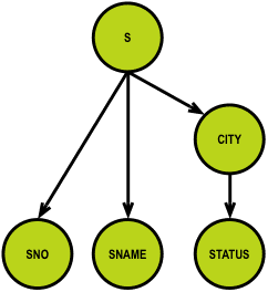
This could have been more pedagogical:

*Inspired by online learning pages from Charles Darwin University, Bob Dewhurst (http://bit.ly/29XOVvD).

Unfortunately, not many people have worked with functional dependencies on the visual level as Bob Dewhurst does in the diagram above.

In his seminal book “Introduction to Database Systems, Volume I”, C.J. Date creates little “FD diagrams” that show the relationships between attributes in relations. The attributes are each in small rectangles (similar to concept maps), but the relationships are not named.

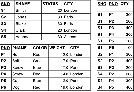
Beyond functional dependencies, other spill-overs from normalization include avoiding redundancies and update anomalies. Date‘s famous supplier-parts example illustrates this:

This is in second normal form, which implies that it could contain redundancy (of city, for example). It also implies an update anomaly; it is impossible to register a city before you have a supplier in that city. City and Supplier are more independent than dependent. Supplier No (SNO) is not an identifying key for Cities. But, yes, there is a relationship between Supplier and City, but having them in the same relation is not a good idea, because it hides important structural information (the relationship between supplier and city).

This relation is ill-defined because not all of its fields are functionally dependent on the same key. So, what the cookbook recipe of normalization is doing is identifying which relations (tables) are not well-formed (according to the mathematics behind the paradigm used by Dr. Ted Codd in his relational model).

Since the co-location is only on the visual level (in the logical data model), and since the physical model might be more or less granular than the tabular model (e.g. in a graph database or denormalized), normalization per se looses importance these days as a vehicle for eliminating physical redundancies and anomalies. However, normalization was also designed to help identifying the inherent (business defined) structures, and that remains a key obligation of the data modeler.

Detecting dependencies is still very important. One advantage of graph databases is that they make dependencies very visible. Here is a simple directed graph model representation of the ill-formed relation above:

Visualization of functional dependencies is certainly a business requirement of data modeling. It’s a powerful tool for detecting dependencies and many more processes. This is why I call it “The Power of Dependencies”!

To reflect a bit on the challenges that the relational model brought upon us, I will first turn your attention to the term “relation.”

What the term “relation” implies (loosely) is that the relation is a set of binary relations, and if all those relations are functionally dependent on the same function, the functional relation of all of the set members (or columns) is good to go; properly normalized. Many people think “relationship” when they hear the term “relation.”

Data modelers are looking for structure, but relationships are secondary citizens of relational. They are normally not named at all in the visualizations and functional dependencies, leading to a loss of meaning / semantics. This goes for both inter-table and intra-table dependencies.

Directed graphs excel in visualizing relationships. Can we turn our table models into graphs? Let us revisit with the Chris Date-style supplier/parts (SP) relations (relvars), and transform them into a proper solution model in five easy steps. The relvars are called S (suppliers), P (parts), and SP (supplier/parts). Here they are, in tabular form:

STEP 1: Draw a naive concept map of S, P, and SP:

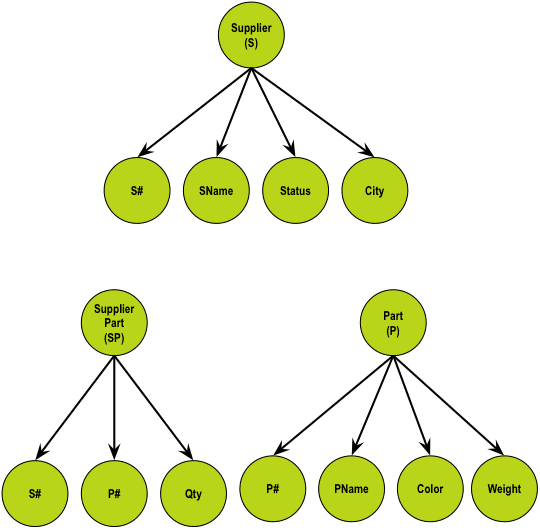
Note that this is just to get us started; no particular symbolism is needed in the representation yet.

STEP 2: Visualize the relationships between S, P, and SP:

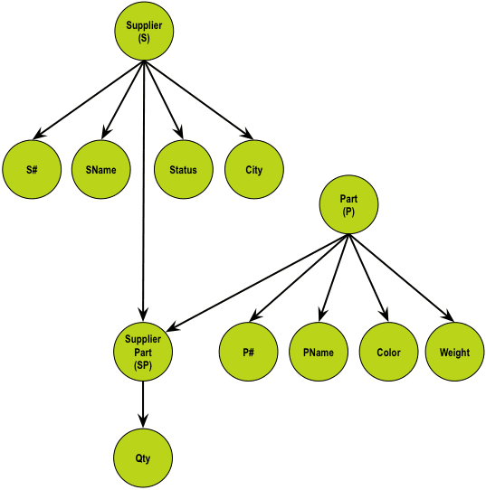
There is indeed a many-to-many relationship between S and P—only carrying the Qty as information. The foreign keys of supplier-part are S# and P#, because they are the identities of S and P, respectively.

STEP 3: Name the relationships:

Naming the relationships adds a new level of powerful information. Some relationships are rather vague (using the verb “has,” for example). Other relationships are much more business-specific (for example, “supplies.”) The data modeler must work with the business to find helpful, specific names for the relationships.

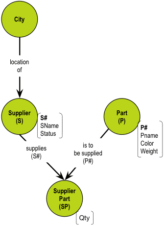
The presence of a verb in the relationship between supplier and city could well mean that it is not a straightforward property relationship. In fact, cities do not share identity with suppliers; suppliers are located in cities. (This is how to resolve functional dependencies.)

STEP 4: Resolving the functional dependency of city:

STEP 5: Reducing to a property graph data model:

Concepts, which are demonstrably the end nodes of (join) relationships between business objects, have been marked in bold. These were originally highlighted in the relationship name (“identified by”). This bold notation corresponds to C. J. Date‘s original syntax in his presentations, where primary key columns had a double underscore under the attribute name.

All concepts in the preceding concept map, which have simple relationships (has, is …), and which only depend on the one and same referencing concept, have been reduced to properties (attributes, if you insist).

The rationale for relational normalization was not clearly stated from a business perspective, but it the benefits were clearly related to identity and uniqueness.

These issues are at the logical level of a solution model. But why do we need to worry about this? The trouble is that we humans do not really care about uniqueness. What is in a name, anyway? We all know that “James Brown” can refer to a very large number of individuals. The trick is to add context: “Yes, you know, James Brown, the singer and the Godfather of Soul.” When uniqueness really matters, context is the definite answer.

The requirement for unique identification is, then, an IT-driven necessity. This gave rise to the “artificial” identifiers (Social Security Number, for example) on the business level and the ID fields (surrogate keys) on the database level. We, as data modelers, must handle these difficult issues in a consistent manner across:

• Identity
• Uniqueness
• Context

This reflects the observation that uniqueness is based on “location” in the meaning of “multi-dimensional coordinates” with a specific context.

The end result is that identity is derived from uniqueness, which sets the context.

The relational discussion started sort of backwards. Much of the discussion about candidate keys is based on the assumption that the problem to be solved is structured as follows:

• Here is a “relation” (a list of fields, really) having these attribute names (S#, SNAME, etc.)
• What could possibly be the candidate keys?
• What is the quality (uniqueness, I guess) of those keys?

But that is a very awkward starting point. Why pick that particular permutation, out of all the concepts that could eventually contribute to a “well-formed” (normalized) relation? Even if your starting point is a report or a screen mockup, you immediately start to go for the structure (graph it); identity and uniqueness will “fall out of the sky” as you go along.

Functional dependency theory needs to be made simpler. And visualization is the answer.