
Click to learn more about author Rosaria Silipo.

The co-author of this column was Kathrin Melcher.
Decision trees are a set of very popular supervised classification algorithms. They are very popular for a few reasons: They perform quite well on classification problems, the decisional path is relatively easy to interpret, and the algorithm to build (train) them is fast and simple.
There is also an ensemble version of the decision tree: the random forest. The random forest essentially represents an assembly of a number N of decision trees, thus increasing the robustness of the predictions.
In this article, we propose a brief overview of the algorithm behind the growth of a decision tree, its quality measures, the tricks to avoid overfitting the training set, and the improvements introduced by a random forest of decision trees.
What Is a Decision Tree?
A decision tree is a flowchart-like structure made of nodes and branches (Fig. 1). At each node, a split on the data is performed based on one of the input features, generating two or more branches as output. More and more splits are made in the upcoming nodes and increasing numbers of branches are generated to partition the original data. This continues until a node is generated where all or almost all of the data belong to the same class and further splits — or branches — are no longer possible.
This whole process generates a tree-like structure. The first splitting node is called the root node. The end nodes are called leaves and are associated to a class label. The paths from root to leaf produce the classification rules. If only binary splits are possible, we talk about binary trees. Here, however, we want to deal with the more generic instance of non-binary decision trees.
Let’s visualize this with an example. We collected data about a person’s past sailing plans, i.e., whether or not the person went out sailing, based on various external conditions — or “input features” — e.g., wind speed in knots, maximum temperature, outlook, and whether or not the boat was in winter storage. Input features are often also referred to as non-target attributes or independent variables. We now want to build a decision tree that will predict the sailing outcome (yes or no). The sailing outcome feature is also known as either the target or the dependent variable.
If we knew about the exact classification rules, we could build a decision tree manually. But this is rarely the case. What we usually have are data: the input features on one side and the target feature to predict on the other side. A number of automatic procedures can help us extract the rules from the data to build such a decision tree, like C4.5, ID3 or the CART algorithm (J. Ross Quinlan). In all of them, the goal is to train a decision tree to define rules to predict the target variable, which in our example is whether or not we will go sailing on a new day.
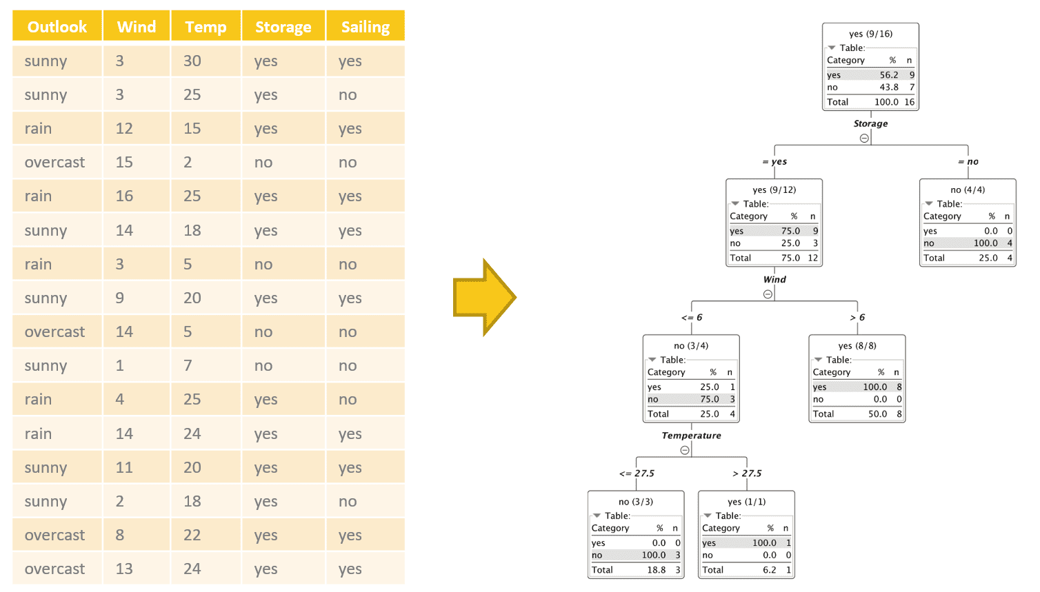
Figure 1. Example of a decision tree (on the right) built on sailing experience data (on the left) to predict whether or not to go sailing on a new day.
Building a Decision Tree
Let’s explore how to build a decision tree automatically, following one of the algorithms listed above.
The goal of any of those algorithms is to partition the training set into subsets until each partition is either “pure” in terms of target class or sufficiently small. To be clear:
- A pure subset is a subset that contains only samples of one class.
- Each partitioning operation is implemented by a rule that splits the incoming data based on the values of one of the input features.
Summarizing, a decision tree consists of three different building blocks: nodes, branches and leaves. The nodes identify the splitting feature and implement the partitioning operation on the input subset of data; the branches depart from a node and identify the different subsets of data produced by the partitioning operation; and the leaves, at the end of a path, identify a final subset of data and associate a class with that specific decision path.
In the tree in figure 1, for example, the split in the first node involves the “Storage” feature and partitions the input subset into two subsets: one where Storage is “yes” and one where Storage is “no.” If we follow the path for the data rows where Storage = yes, we find a second partitioning rule. Here the input dataset is split in two datasets: one where “Wind” > 6 and one where “Wind” <= 6. How does the algorithm decide which feature to use at each point to split the input subset?
The goal of any of these algorithms is to recursively partition the training set into subsets until each partition is as pure as possible in terms of output class. Therefore, at each step, the algorithm uses the feature that leads to the purest output subsets.
Quality Measures
At each iteration, in order to decide which feature leads to the purest subset, we need to be able to measure the purity of a dataset. Different metrics and indices have been proposed in the past. We will describe a few of them here, arguably the most commonly used ones: information gain, Gini index, and gain ratio.
During training, the selected quality measure is calculated for all candidate features to find out which one will produce the best split.
Entropy
Entropy is a concept that is used to measure information or disorder. And, of course, we can use it to measure how pure a dataset is.
If we consider the target classes as possible statuses of a point in a dataset, the entropy of a dataset can be mathematically defined as the sum over all classes of the probability of each class multiplied by the logarithm of it. For a binary classification problem, thus, the range of the entropy falls between 0 and 1.

Where p is the whole dataset, N is the number of classes, and pi is the frequency of class i in the same dataset.
To get a better understanding of entropy, let’s work on two different example datasets, both with two classes, respectively represented as blue dots and red crosses (Fig. 2). In the example dataset on the left, we have a mixture of blue dots and red crosses. In the example of the dataset on the right, we have only red crosses. This second situation — a dataset with only samples from one class — is what we are aiming at: a “pure” data subset.
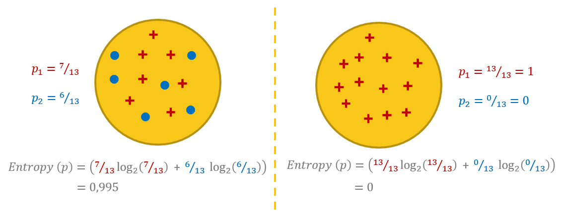
Figure 2. Two classes: red crosses and blue dots. Two different datasets. A dataset with a mix of points belonging to both classes (on the left) and a dataset with points belonging to one class only (on the right).
Let’s now calculate the entropy for these two binary datasets.
For the example on the left, the probability is 7/13 for the class with red crosses and 6/13 for the class with blue dots. Notice that here we have almost as many data points for one class as for the other. The formula above leads to an entropy value of 0.99.
For the example on the right, the probability is 13/13 = 1.0 for the class with the red crosses and 0/13 = 0.0 for the class with the blue dots. Notice that here we have only red cross points. In this case, the formula above leads to an entropy value of 0.0.
Entropy can be a measure of purity, disorder or information. Due to the mixed classes, the dataset on the left is less pure and more confused (more disorder, i.e., higher entropy). However, more disorder also means more information. Indeed, if the dataset has only points of one class, there is not much information you can extract from it no matter how long you try. In comparison, if the dataset has points from both classes, it also has a higher potential for information extraction. So, the higher entropy value of the dataset on the left can also be seen as a larger amount of potential information.
The goal of each split in a decision tree is to move from a confused dataset to two (or more) purer subsets. Ideally, the split should lead to subsets with an entropy of 0.0. In practice, however, it is enough if the split leads to subsets with a total lower entropy than the original dataset.
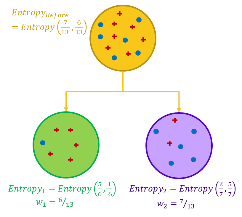
Figure 3. A split in a node of the tree should move from a higher entropy dataset to subsets with lower total entropy.
Information Gain (ID3)
In order to evaluate how good a feature is for splitting, the difference in entropy before and after the split is calculated.
That is, first we calculate the entropy of the dataset before the split, and then we calculate the entropy for each subset after the split. Finally, the sum of the output entropies weighted by the size of the subsets is subtracted from the entropy of the dataset before the split. This difference measures the gain in information or the reduction in entropy. If the information gain is a positive number, this means that we move from a confused dataset to a number of purer subsets.

Where “before” is the dataset before the split, K is the number of subsets generated by the split, and (j, after) is subset j after the split.
At each step, we would then choose to split the data on the feature with the highest value in information gain as this leads to the purest subsets. The algorithm that applies this measure is the ID3 algorithm. The ID3 algorithm has the disadvantage of favoring features with a larger number of values, generating larger decision trees.
Gain Ratio (C4.5)
The gain ratio measure, used in the C4.5 algorithm, introduces the SplitInfo concept. SplitInfo is defined as the sum over the weights multiplied by the logarithm of the weights, where the weights are the ratio of the number of data points in the current subset with respect to the number of data points in the parent dataset.
The gain ratio is then calculated by dividing the information gain from the ID3 algorithm by the SplitInfo value.

Where “before” is the dataset before the split, K is the number of subsets generated by the split, and (j, after) is subset j after the split.
Gini Index (CART)
Another measure for purity — or actually impurity — used by the CART algorithm is the Gini index.
The Gini index is based on Gini impurity. Gini impurity is defined as 1 minus the sum of the squares of the class probabilities in a dataset.

Where p is the whole dataset, N is the number of classes, and pi is the frequency of class i in the same dataset.
The Gini index is then defined as the weighted sum of the Gini impurity of the different subsets after a split, where each portion is weighted by the ratio of the size of the subset with respect to the size of the parent dataset.
For a dataset with two classes, the range of the Gini index is between 0 and 0.5: 0 if the dataset is pure and 0.5 if the two classes are distributed equally. Thus, the feature with the lowest Gini index is used as the next splitting feature.

Where K is the number of subsets generated by the split and (j, after) is subset j after the split.
Identifying the Splits
For a nominal feature, we have two different splitting options. We can either create a child node for each value of the selected feature in the training set, or we can make a binary split. In the case of a binary split, all possible feature value subsets are tested. In this last case, the process is more computationally expensive but still relatively straightforward.
In numerical features, identifying the best split is more complicated. All numerical values could actually be split candidates. But this would make computation of the quality measures too expensive an operation! Therefore, for numerical features, the split is always binary. In the training data, the candidate split points are taken in between every two consecutive values of the selected numerical feature. Again, the binary split producing the best quality measure is adopted. The split point can then be the average between the two partitions on that feature, the largest point of the lower partition or the smallest point of the higher partition.
Size and Overfitting
Decision trees, like many other machine learning algorithms, are subject to potentially overfitting the training data. Trees that are too deep can lead to models that are too detailed and don’t generalize on new data. On the other hand, trees that are too shallow might lead to overly simple models that can’t fit the data. You see, the size of the decision tree is of crucial importance.
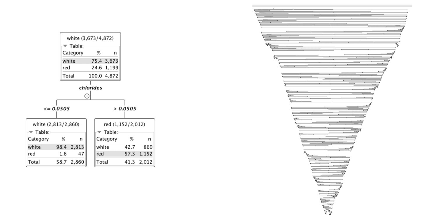
Figure 4. The size of the decision tree is important. A tree that is large and too detailed (on the right) might overfit the training data, while a tree that is too small (on the left) might be too simple to fit the data.
There are two ways to avoid an over-specialized tree: pruning and/or early stopping.
Pruning
Pruning is applied to a decision tree after the training phase. Basically, we let the tree be free to grow as much as allowed by its settings, without applying any explicit restrictions. At the end, we proceed to cut those branches that are not populated sufficiently so as to avoid overfitting the training data. Indeed, branches that are not populated enough are probably overly concentrating on special data points. This is why removing them should help generalization on new unseen data.
There are many different pruning techniques. Here, we want to explain the two most commonly used: reduced error pruning and minimum description length pruning, MDL for short.
In reduced error pruning, at each iteration, a low populated branch is pruned and the tree is applied again to the training data. If the pruning of the branch doesn’t decrease the accuracy on the training set, the branch is removed for good.
MDL pruning uses description length to decide whether or not to prune a tree. Description length is defined as the number of bits needed to encode the tree plus the number of bits needed to encode the misclassified data samples of the training set. When a branch of the tree is pruned, the description lengths of the non-pruned tree and of the pruned tree are calculated and compared. If the description length of the pruned tree is smaller, the pruning is retained.
Early Stopping
Another option to avoid overfitting is early stopping, based on a stopping criterion.
One common stopping criterion is the minimum number of samples per node. The branch will stop its growth when a node is created containing fewer or an equal number of data samples as the minimum set number. So a higher value of this minimum number leads to shallower trees, while a smaller value leads to deeper trees.
Random Forest of Decision Trees
As we said at the beginning, an evolution of the decision tree to provide a more robust performance has resulted in the random forest. Let’s see how the innovative random forest model compares with the original decision tree algorithms.
Many is better than one. This is, simply speaking, the concept behind the random forest algorithm. That is, many decision trees can produce more accurate predictions than just one single decision tree by itself. Indeed, the random forest algorithm is a supervised classification algorithm that builds N slightly differently trained decision trees and merges them together to get more accurate and stable predictions.
Let’s stress this notion a second time. The whole idea relies on multiple decision trees that are all trained slightly differently and all of them are taken into consideration for the final decision.
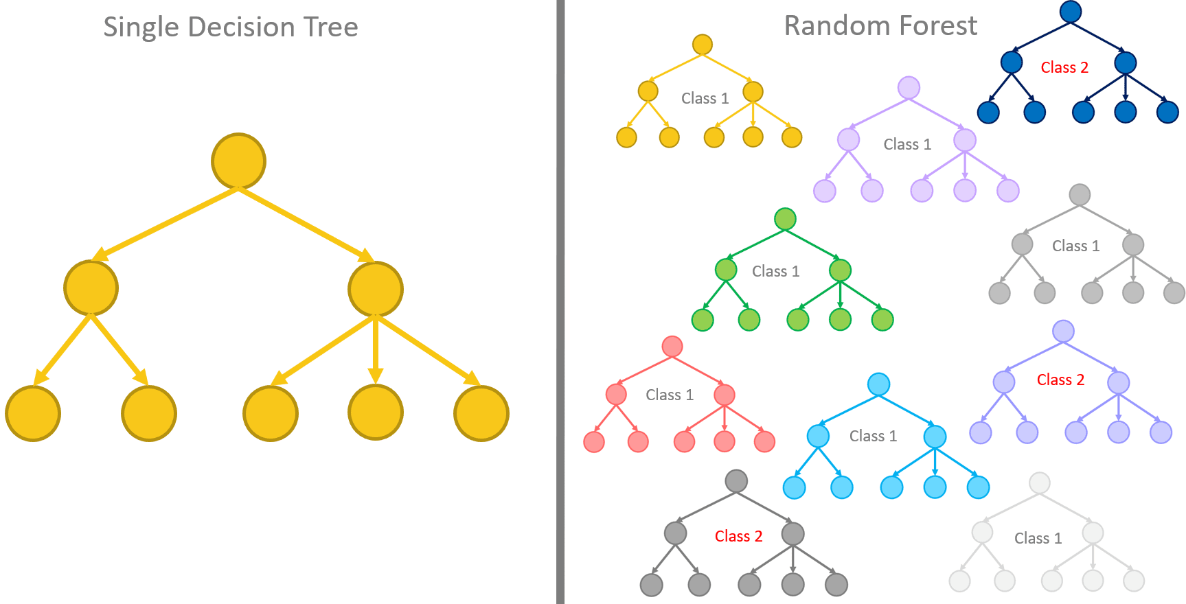
Figure 5. The random forest algorithm relies on multiple decision trees that are all trained slightly differently; all of them are taken into consideration for the final classification.
Bootstrapping of Training Sets
Let’s focus on the “trained slightly differently.”
The training algorithm for random forests applies the general technique of bagging to tree learners. One decision tree is trained alone on the whole training set. In a random forest, N decision trees are trained each one on a subset of the original training set obtained via bootstrapping of the original dataset, i.e., via random sampling with replacement.
Additionally, the input features can also be different from tree to tree, as random subsets of the original feature set. Typically, if m is the number of the input features in the original dataset, a subset of randomly extracted [square root of m] input features is used to train each decision tree.
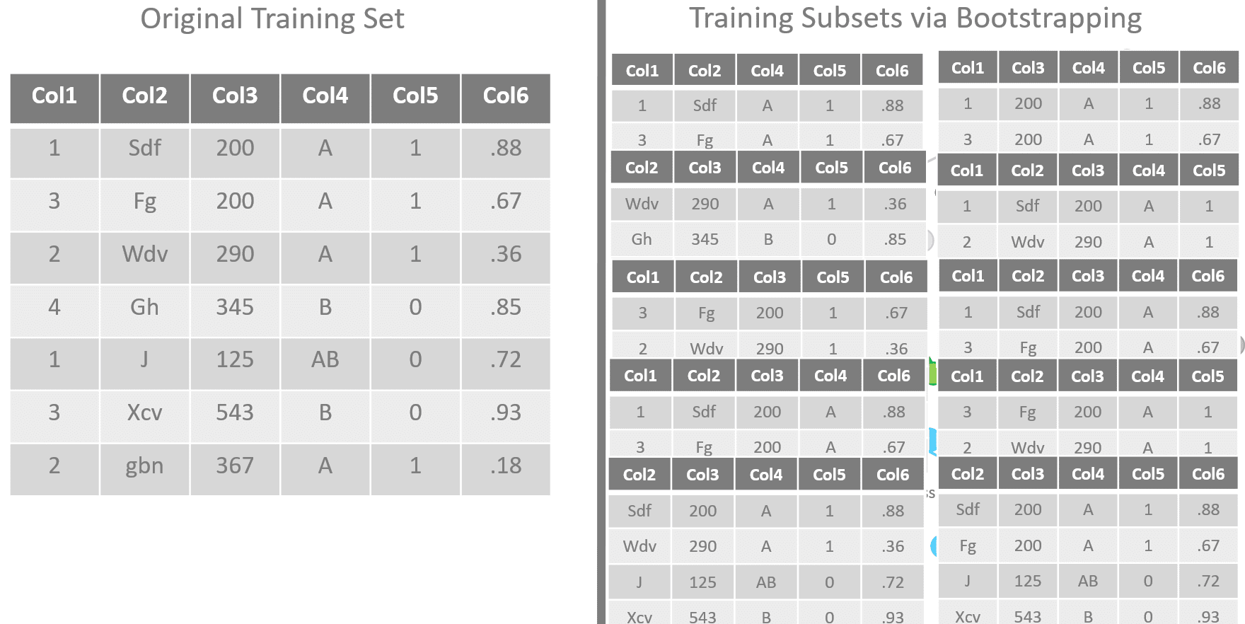
Figure 6. The decision trees in a random forest are all slightly differently trained on a bootstrapped subset of the original dataset. The set of input features also varies for each decision tree in the random forest.
The Majority Rule
The N slightly differently trained trees will produce N slightly different predictions for the same input vector. Usually, the majority rule is applied to make the final decision. The prediction offered by the majority of the N trees is adopted as the final one.
The advantage of such a strategy is clear. While the predictions from a single tree are highly sensitive to noise in the training set, predictions from the majority of many trees are not — providing the trees are not correlated. Bootstrap sampling is the way to decorrelate the trees by training them on different training sets.
Out of Bag (OOB) Error
A popular metric to measure the prediction error of a random forest is the out-of-bag error.
Out-of-bag error is the average prediction error calculated on all training samples xᵢ, using only the trees that did not have xᵢ in their bootstrapped training set. Out-of-bag error estimates avoid the need for an independent validation dataset but might underestimate actual performance improvement.
Conclusions
In this article, we reviewed a few important aspects of decision trees: how a decision tree is trained to implement a classification problem, which quality measures are used to choose the input features to split, and the tricks to avoid the overfitting problem.
We have also tried to explain the strategy of the random forest algorithm to make decision tree predictions more robust; that is, to limit the dependence from the noise in the training set. Indeed, by using a set of N decorrelated decision trees, a random forest increases the accuracy and the robustness of the final classification.
Now, let’s put it to use and see whether we will be going sailing tomorrow!
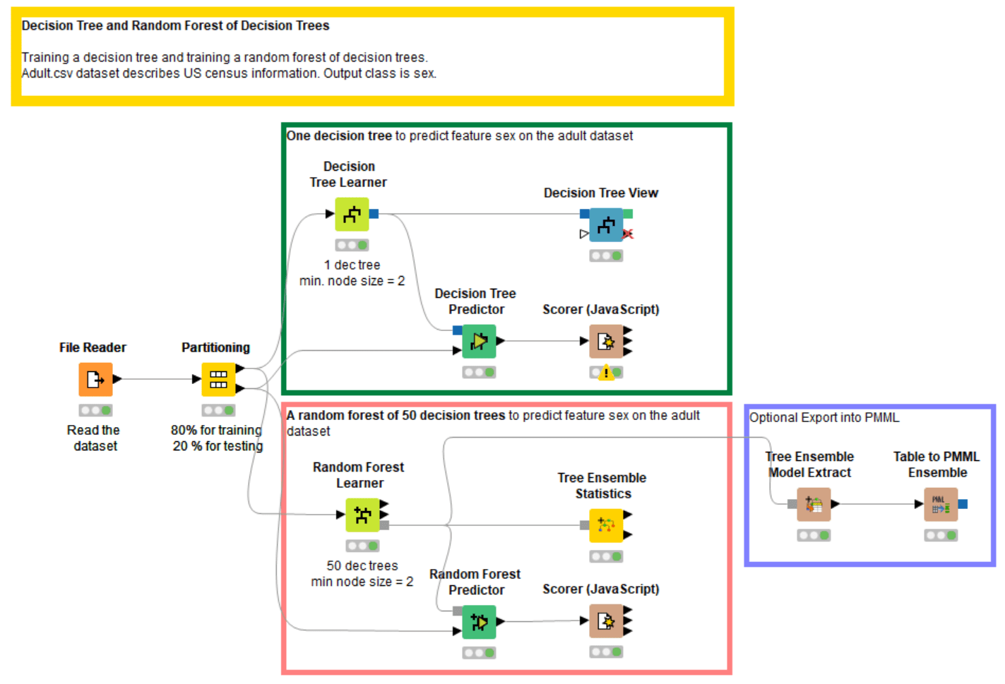
Figure 7. The workflow implementing the training and evaluation of a decision tree and of a random forest of decision trees. This workflow can be inspected and downloaded from the KNIME Hub at https://kni.me/w/Eot69vL_DI5V79us.
Reference
J. Ross Quinlan, “C4.5: Programs for Machine Learning,” Morgan Kaufmann Publishers Inc., San Francisco, CA USA ©1993
Appendix
You can find an example of how to train and evaluate a decision tree and a random forest of decision trees on the KNIME Open Source Hub at https://kni.me/w/Eot69vL_DI5V79us. This workflow is also shown in figure 7.