
Click to learn more about author Paolo Tamagnini.
In this second article of our integrated deployment blog series – where we focus on solving the challenges around productionizing Data Science – we look at the model part of the process.
In the previous article we covered a simple integrated deployment use case. We first looked at an existing pair of workflows, one that created a model and the second that used that model for production. Then we looked at how to build a model workflow that automatically creates a workflow that can be used in production immediately. To do this, we used the new Integrated Deployment Extension. That first scenario was quite simple. Things can get more complicated quickly, however, in a real situation.
For example, how would the workflow using integrated deployment look if we were training more than one model? How would we flexibly deploy the best one? Assuming that we have to test the training and deployment workflow on a subset of the data, how would we then retrain and redeploy on a bigger dataset by picking only the interesting pieces of the initial workflow? Let’s see how integrated deployment can help us accomplish these tasks.
To be able to train multiple models, select the best one, retrain it again, and automatically deploy it, we would want to make a hierarchy of workflows: the modeling workflow that generates the training workflow that generates the deployment workflow (Figure 1).
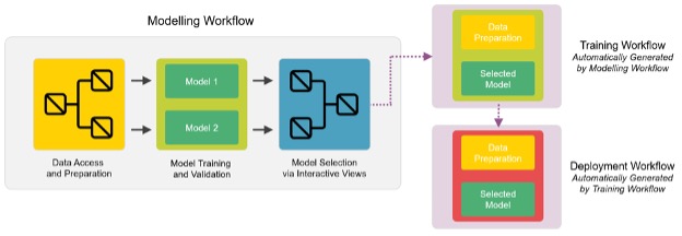
Figure 1: A diagram explaining the hierarchical structure of workflows necessary to build an application for selecting the best model and retraining and deploying it on the fly.
The entire system can be controlled and edited from the modeling workflow thanks to integrated deployment. By adding Capture Workflow nodes (Capture Workflow Start and Capture Workflow End) the data scientist is able to select which nodes to use to retrain the selected model and which nodes to deploy it. Furthermore using switches like Case Switch nodes and Empty Table Switch node the data scientist can define the logic on what node should be captured and added to the other two workflows.
Using the framework depicted in Figure 1 becomes especially useful in a business scenario where retraining and redeploying a variety of models takes place in a routine fashion. Without such a framework the data scientist would be required to manually intervene on the workflows each time the deployed model needs to be retrained with different settings.
In Figure 2 an animation shows the modeling workflow – with integrated deployment used to capture and execute on demand the training workflow and finally write only the deployment workflow.

The workflow goes through a standard series of steps to create multiple models, in this case a Random Forest and an XGBoost Model. It then offers an interactive view so that a data scientist can investigate the results and decide which model should be retrained on more data and finally deployed. It covers the steps of the CRISP-DM cycle and in addition offers interactive views to the user. The user can select which workflow should be retrained on more data and finally deployed.
At this point, you might feel a bit overwhelmed. It’s like that 2010 movie about a dream within a dream, “Inception.” If that is the case, do not worry – it will get better.
We will walk through each part of the workflow and display them here. You might find it more helpful to have the example open as you follow along. Remember to have KNIME 4.2 or later installed! The example workflow can be found here.
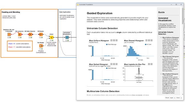
We start by accessing some data as usual from a database and a CSV file and blending them. At this point the data scientist is looking at the data via an interactive composite view called Automated Visualization (Figure 3). This view offers the data scientist a quick way to look at anomalies via a number of charts that automatically display what is most interesting statistically.
Once that is done the data scientist builds the custom process to prepare the data for the analytics process. In this example we are just going to update the domain of all columns and convert a few columns from numerical to categorical. The data scientist captures the workflow with integrated deployment because it will be needed in the future where more data is to be processed. In our example, the data scientist then opens an Interactive Column Filter Component. This view allows for the quick removal columns, which should not be used by the model for all the normal reasons such as too many missing, constant or unique values (Figure 4).
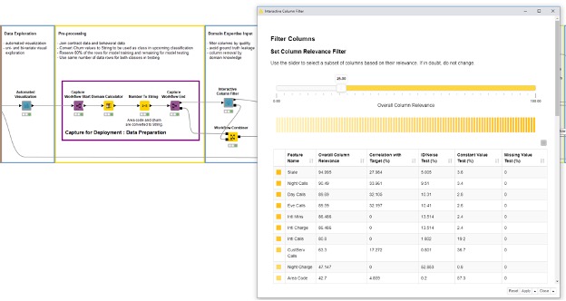
Figure 4: The modeling workflow continues with the data preparation part, which is captured for later deployment. Another interactive view is used to filter out irrelevant columns quickly before the training of the models. Also the interactive filter is captured for deployment purposes.
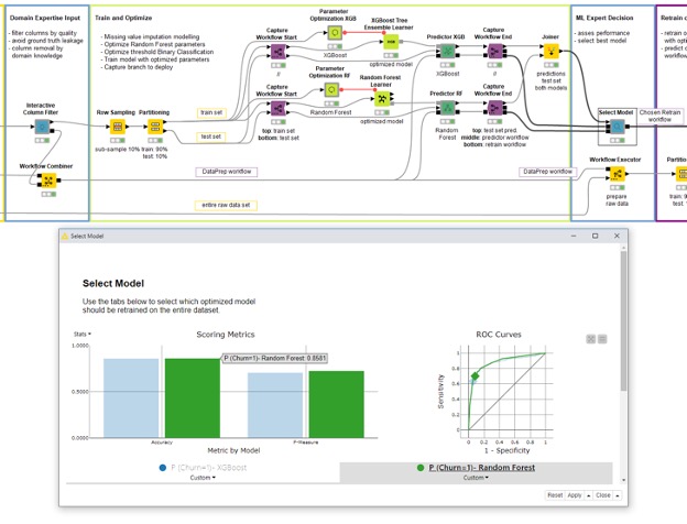
This data scientist in particular is dealing with an enormous amount of rows. To perform model optimization quickly she wants to subsample the data with a Row Sampling node to use only 10%. The data scientist knows she will need to retrain everything afterwards with more data to get accurate results but for the time being is happy with 10%. After splitting the sub-sampled data into train and test sets, she trains an XGBoost Model and a Random Forest model with Parameter Optimization on top. To retrain later the data scientist also captures this part with integrated deployment. After training the two models she uses yet another interactive view to see which model is better (Figure 5). The chosen model is Random Forest, which is automatically selected at the Workflow Object port by the Component.
The selected model is retrained on the entire dataset (no 10% subsampling this time) with a Workflow Executor node using the output of the previous component. The previous component produces a training workflow (Figure 6). When executing the training workflow, the output from its Workflow Executor node is the deployment workflow (Figure 6). And there you have it: a complete and automated example of continuous deployment! Hopefully you don’t have that overwhelmed feeling anymore.

The deployment workflow and the scored new test set is used in the last interactive view (Figure 7) to see the new performance, as this time more data was used. Two buttons are provided: The first one enables the download for the deployment workflow in .knwf format, the second one offers the ability to deploy it to the Server and save a local copy of the produced deployment workflow.
This same workflow can be deployed to the WebPortal via the Server as an interactive Guided Analytics application. The application can be used by data scientists whenever they need to go through a continuous deployment cycle – which, in effect, is a tight, custom, and interactive AutoML application. Of course, this particular application is hard-coded for this particular machine learning use case, but you can modify this example to suit your needs.
Stay tuned for the next installment of the integrated deployment blog series, where we show how to use integrated deployment for a more complete and flexible AutoML solution.