Click here to learn more about Steve Miller.
Toward the end of last month’s blog on SAS, R, Python, and WPS, I mentioned a current project challenge of identifying and eliminating “mostly” null columns from wide SAS data sets. As the team discovered, such columns can impose a significant drag on performance. My take is that while finding empty columns in SAS is easy, removing them is another matter. Touting the emerging interoperability among SAS, R, and Python, I noted that one solution to the problem involved pulling the SAS data sets into R data.frames (or data.tables), identifying the offending columns, creating new data.frames absent those columns, and then pushing the revised data.frames back into SAS. Not exactly elegant, but workable.
Not only did someone actually read the recommendation, but also asked if I’d share the R thinking. So here we are. From a point of departure of an R data.frame “pulled” from WPS/SAS, what follows is high level R code in a jupyter notebook to first explore, then to identify and remove “mostly empty” columns from wide data sets. The test data consists of 1,642,901 records with 264 columns, the majority of which it turns out are nearly empty and therefore not useful for analysis.First, invoke the driving R packages, set a few options, and load the data.table in manner that mimics WPS’s proc R. Interrogate the resulting data structure dimensions.
First, invoke the driving R packages, set a few options, and load the data.table in manner that mimics WPS’s proc R. Interrogate the resulting data structure dimensions.

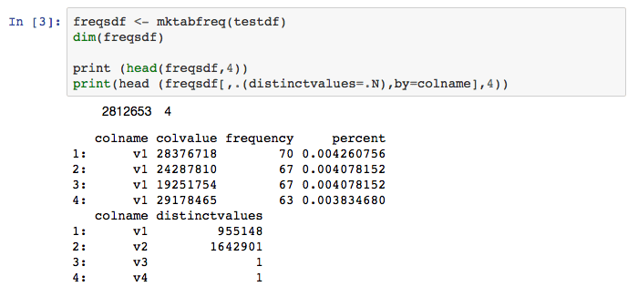
Next, define two functions using data.table to compute frequencies that’ll elucidate the empty column problem. The first function tabulates frequencies for a single column using data.table’s elegant syntax; the second function calls the first for every column in the table. The “output” is a data.table that stacks the frequencies of each column. This table can become quite “long”, since there’s a row for each distinct value of every column.

Now invoke the mktabfreq function on the testdf data.table. Print the frequency table along with a summary that delineates the number of distinct values for each table column. Lots of 1’s in the number of distinct values is an indication of a substantial empty column problem — a finding indeed confirmed by the function calls. Several records from each table are displayed.
Next define a function to compute the number and proportion of missing values for each data.table column. The function must handle NAs for all data types in addition to identifying character vars consisting of all white space as NA. A data.table is returned noting the column name, its length, the number of “missings”, and the proportion of missings.

Run the mkpctnull function on the testdf data.table, generating the missing data report. With a threshold of permissable not null values arbitrarily set to 15%, determine how many and which columns pass by querying the nullrepdf data.table. Compute a new data.table, testdfincl, with only those columns that pass the threshold. Finally, compare the size of the abbreviated data.table with the original and save the reduced data set for subsequent return to SAS/WPS.
In this case with a not null minimum of 15%, only 31 of the 264 original columns survive, a data.table size decrease of over 75%. In the larger WPS/R app, this reduced data.table is then pushed back into WPS for further SAS language processing.

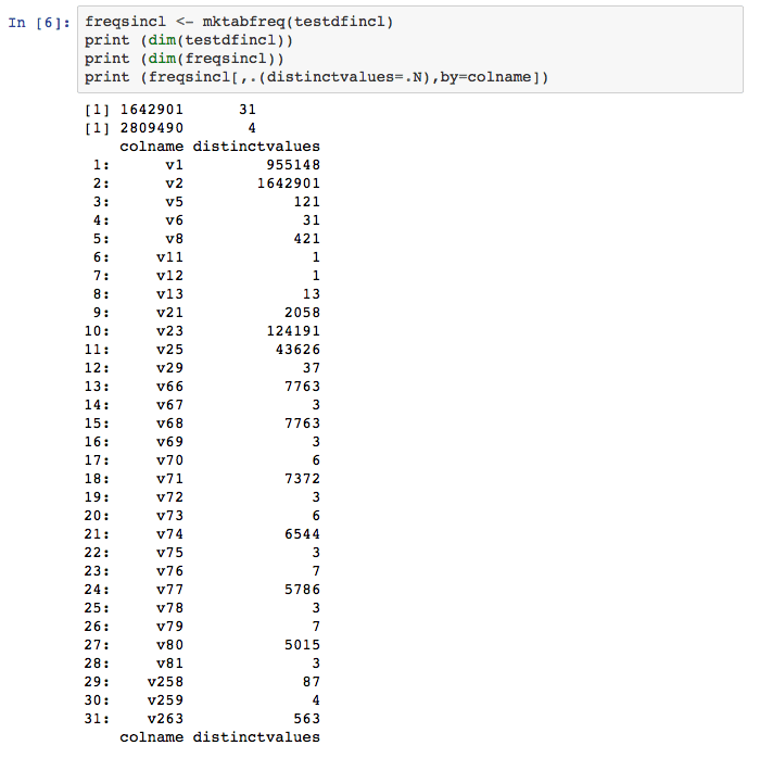
Finally, take a look at the number of distinct values of the reduced 31 attribute data.frame.
I’ll have more to say on the collaboration of R, Python, and SAS/WPS in coming blogs.