“Garbage in, garbage out” defines the importance of data in data science or machine learning in a nutshell. Incorrect input will yield meaningless results and screening data ensures we get comprehensible results. Before we start building models and generating insights, we need to ensure that the quality of the data we are working with is as close to flawless as possible. This is where data screening and checking for assumptions in regression become very crucial for all data scientists.

Screening the data involves looking for characteristics of the data that aren’t directly related to the research questions but could have an impact on how the results of statistical models are interpreted or on whether or not the analysis strategy needs to be revised. This involves taking a close look at how variables and missing values are distributed. The ability to recognize relationships between variables is useful for making modeling choices and interpreting the outcomes.

There are various steps of data screening such as validating data accuracy and checking for missing data and outliers. But one very critical aspect of data screening is checking for assumptions. Parametric statistics relies substantially on assumptions, which establish the groundwork for the application and comprehension of statistical models and tests.

Assumptions regarding the underlying distribution of the population or the relationship between the variables under study are necessary for the use of parametric statistics. These presumptions allow data scientists to derive plausible inferences from their data. The accuracy and reliability of statistical approaches are bolstered by the use of reasonable assumptions.

Parametric models establish the features of the population under study by specifying assumptions and providing a framework for estimating population parameters from sample data. Statistical methods like analysis of variance (ANOVA) and linear regression have assumptions that must be met to get reliable results.

In this article, we will go over the various assumptions one needs to meet in regression for a statistically significant analysis. One of the first assumptions of linear regression is independence.

Independence Assumption 

Independence assumption specifies that the error terms in the model should not be related to each other. In other words, the covariance between the error terms should be 0 and can be represented as 

It’s critical to satisfying independence assumption, as violating it would mean that confidence intervals and significance tests will be invalid for the analysis. In the case of time series data where we often have scenarios with data being temporally correlated, violating the independence assumption may lead to bias in parameter estimation for regression and provide invalid statistical inferences. 

Additivity Assumption

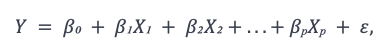
In linear regression, the additivity assumption simply says that when there are multiple variables, their total influence on the outcome is best stated by combining their effects together (i.e., the effect of each predictor variable on the outcome variable is additive and independent of other predictors). For a multiple linear regression model, we can represent the above statement mathematically as follows, where Y is the outcome variable, X₁, X₂, …, Xₚ are the independent variables or the predator variables, and β₀, β₁, β₂, …, βₚ are their corresponding coefficients, with ε being the error term.

If some of the predictor variables are not additive, then it implies that the variables are too related to each other (i.e., multicollinearity exists, which in turn reduces the model’s predictive power).

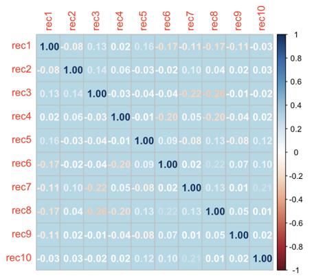
In order to validate this assumption, you can plot the correlation between the predictor variables. In Figure 1, we observe a correlation plot between 10 predictor variables. If we observe the figure none of the variables have a significant correlation between them (i.e., above 80). Hence, we can confirm that for this particular case, the additivity assumption is satisfied. However, if they were too high among a set of variables then you can either combine them or just use one of them in your study.

Linearity Assumption

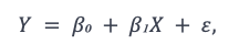
In linear regression, the linearity assumption states that the predictor variables and the outcome variable share a linear relationship between them. For a simple linear regression model, we can represent this mathematically as follows where Y is the outcome variable, X is the predictor variable, β₁ is its coefficient and β₀ is the intercept with ε being the error term.

We usually evaluate residual plots, such as scatterplots of residuals against anticipated values or predictor variables or a normal quantile-quantile (q-q norm) plot which helps us determine if two data sets come from populations with a common distribution, to assess linearity. Nonlinear patterns in these plots suggest that the linearity assumption has been violated which may lead us to biased parameter estimation and incorrect predictions. Let’s take a look at how we can use a q-q norm plot of standardized errors or residuals in order to validate the linearity assumption.

In Figure 2 we observe how the standardized errors are distributed around 0. Because we are attempting to forecast the outcome of a random variable, errors should be randomly distributed (i.e., a large number of small values centered on zero). In order to have a comparable scale for all the residuals we standardize the errors resulting in a standard normal distribution. Each dot in the plot represents how a standardized residual is plotted against the theoretical residual for the area of the standardized distribution. We also observe how most of the residual data points are centered around 0 and lie between -2 and 2 as we expect for a standardized normal distribution, thus helping us validate the linearity assumption. 

Normality Assumption

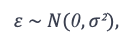
Extending the linearity assumption, we lead to the normality assumption in linear regression which states that the error term or the residual (ε) in the model follows a normal distribution. We can express that mathematically as follows where ε is the error term, N is the normal distribution with 0 being the mean and σ² being the variance.

Satisfying the normality assumption is critical for performing a valid hypothesis testing and accurate estimation of the coefficients. In case the normality test is violated then it might lead to bias in parameter estimation along with inaccurate predictions. In case the error or residual has a skewed distribution then it won’t be able to provide accurate confidence intervals. In order to validate the normality assumption, we can utilize the above q-q norm plot as in Figure 2. Additionally, we can also utilize histograms of standardized errors to validate the normality assumption.

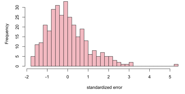
In Figure 3, we observe that the distribution is centered around zero, with most of the data distributed between -2 and 2 which satisfies a standard normal distribution thereby validating the normality assumption.

Homogeneity and Homoscedasticity Assumption

The homogeneity assumption states that the variances of the variables are roughly equal. Meanwhile, the homoscedasticity assumption states that the error term or residual is the same across all values of the independent variables. This assumption is critical, as it makes sure that the errors or residuals do not change with changing values of the predictor variables (i.e., the error term has a consistent distribution). Violating the homoscedasticity assumption, also known as heteroscedasticity, can lead to inaccurate hypothesis testing as well as inaccurate parameter estimation for predictor variables. In order to validate both these assumptions you can create a scatterplot where X-axis values represent standardized predicted values by your regression model and Y-axis values represent standardized residuals or the error terms of your regression model. We need to standardize both these sets of values for an easier scale to interpret. 

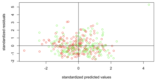
In Figure 4, we observe a scatter plot of standardized predicted values along the x-axis in green and standardized residuals along the y-axis in red. 

We can claim that the homogeneity assumption is satisfied if the spread above the (0,0) line is similar to that below the (0, 0) line in both the x and y directions. In case there is a very large spread on one side and a smaller spread on the other side then we can say that the homogeneity assumption is violated. In the figure, we observe an even distribution across both the lines, and we can claim that the homogeneity assumption is valid for this case.

For homoscedasticity validation, we wish to check if the spread is equal all the way across the x-axis. It should look like an even random distribution of dots. In case the distribution somewhat resembles megaphones, triangles, or big groupings of data then we say that heteroscedasticity is observed. In the figure, we can observe an even random distribution of dots thereby validating the homoscedasticity assumption.

This concludes how we can validate the various assumptions for linear regression and why they are critical. Data scientists can assure the reliability of the regression analysis, generate unbiased estimates, perform valid hypothesis testing, and derive meaningful insights by evaluating and confirming these assumptions.