Click to learn more about author Rosaria Silipo.

Ensemble models combine multiple learning algorithms to improve the predictive performance of each algorithm alone. There are two main strategies to ensemble models — bagging and boosting — and many examples of predefined ensemble algorithms.

Bootstrap aggregation, or bagging, is an ensemble meta-learning technique that trains many classifiers on different partitions of the training data and uses a combination of the predictions of all those classifiers to form the final prediction for the input vector.

Boosting is another committee-based ensemble method. It works with weights in both steps: learning and prediction. During the learning phase, the boosting procedure trains a new model a number of times, each time adjusting the parameters of the new model to the errors of the existing boosted model. During the prediction phase, it provides a prediction based on a weighted combination of the models’ predictions.

Bagging

This ensemble technique was proposed by Breiman in 1994 [1]and can be used with many prediction models.

When we train one single model, the final predictions and model parameters depend on the size and composition of the data partition used for the training set. Especially if the training procedure ends with overfitting [2] the training data, final models and predictions can be very different. We say that in this case the model variance, in terms of parameters and predictions, is very high. Thus, the final effect of the bagging technique is to reduce the model variance and thereby make the prediction process more noise independent.

Bagging Technique Implementation

Tree Ensembles and Random Forest

The most famous ensemble bagging model is definitely the random forest. A random forest is a special type of decision tree ensemble [3].

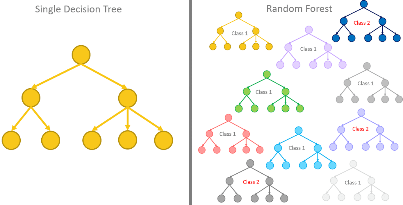
Prepackaged Bagging Models

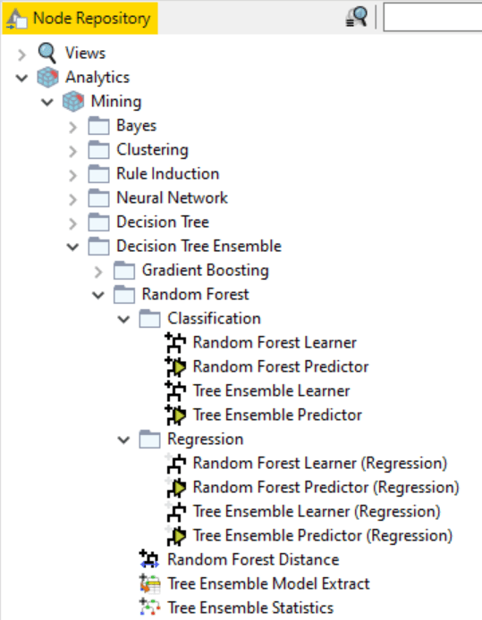
The Analytics Platform has two prepackaged bagging algorithms: the Tree Ensemble Learner and the Random Forest. Both algorithms deal with ensembles of decision trees. The Random Forest though applies the random forest variation to it.

Both node sets refer to a classification set up, which means numerical or categorical/nominal input but only categorical/nominal output for the target class. Working on a classification problem as a supervised model, the implementation relies on the Learner-Predictor motif, as for all other supervised algorithms (Fig. 2).

As far as configuration goes, the Tree Ensemble Learner node allows for the configuration of more free parameters than the Random Forest Learner node. For example, the Tree Ensemble Learner node allows the user to set the number of extracted data samples, the number of input features, and the number of decision trees, while the random forest allows the user only to set the number of decision trees. Both Predictor nodes allow the user to set the majority vote (default) or the highest average probability (soft voting) as the decision strategy for the final class.

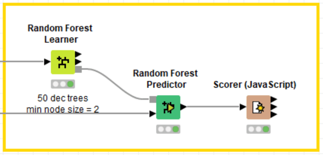
Note the three output ports of both Learner nodes: one is the model (lower port); one is the out-of-bag (OOB) predictions (top port); one is the attribute statistics (in the middle).

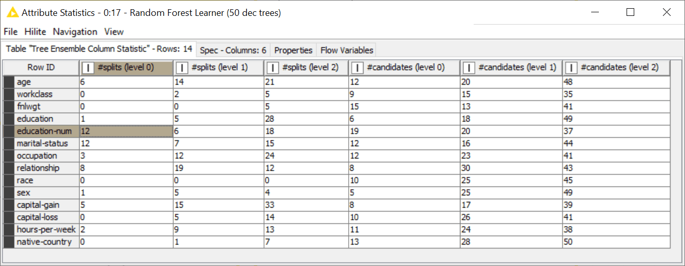
Attribute statistics are useful as a measure of the input feature importance. Indeed, the number of times an attribute is used to split the dataset by the different trees in the ensemble indicates the importance of the attribute. If, for example, “age” is used by many more trees than “gender,” it probably means that its information is more useful to discriminate the classes in the training set. This is even more true if we consider the split level. A split at the very beginning is more general and less prone to overfit the data than a split later on in a tree. So, examining the number of times an attribute has been chosen to split the dataset earlier on in the trees is a good indication of its importance.

Similarly, but to a lower extent, the number of times an attribute has been chosen as a split candidate in the early levels of the trees in the ensemble can be considered a measure of the importance of the input attribute for the final classification.

Notice that similar nodes are available for numerical prediction problems: Random Forest Learner/Predictor (Regression) and Tree Ensemble Learner/Predictor (Regression) nodes.

Custom Bagging Models

Bagging is a general ensemble strategy and can be applied to models other than decision trees. To make your own bagging ensemble model you can use the metanode named “Bagging.”

The Bagging metanode builds the model, i.e., implements the training and testing part of the process. Double-click the metanode to open it. Inside, you can find two loops: The first loop trains the bag of models on the training data; the second loop applies all models to the test data and uses the majority vote (Voting Loop End node) to decide the final class.

This implies a few things:

• Two input ports: one for the training set, one for the test set
• One output port for the predictions on the test set
• Only classification problems, since we use the majority vote as a decision criterion

The default models for the ensemble are decision trees. Any other model could be used as long as the appropriate Learner and Predictor node are placed in the metanode.

The number of models for the ensemble is decided in the Chunk Loop Start node. For N models, the Chunk Loop Start node trains each one of them on a 1/N fraction of the training set. All models are collected by the Model Loop End node. Similarly, all models are retrieved by the Model Loop Start node.

Pieces of the sub-workflow in this metanode could be reused to form the Learner and the Predictor node for the ensemble we want to create.

Boosting

Boosting is another committee-based approach. The idea here is to add multiple weak models at successive steps to refine the prediction task. A weak model is, in general, a light model with few parameters and trained for only a few iterations, for example, a shallow decision tree. Due to its weak character, the model can only perform well on some of the data in the training set. So, at each step, we add one more weak model to focus on the errors of the previous set of models.

This approach has a few advantages. The first one is memory. Small models trained sequentially only for a few iterations on a subset of data require less memory at each step than, for example, a random forest training many stronger models all at the same time. The second advantage is the specialization of the weak models. They might not perform well in general, but they perform well on some types of data. Thus, each one of them can be weighted appropriately in the decision process.

Boosting Technique Implementation

Boosting was introduced for numerical prediction tasks. It is possible to extend it to classification by taking into account the class probabilities as predicted values.

The training set for the first iteration is the whole training set.

The algorithm stops when a maximum number of iterations M has been reached or the model error is too big (that is, the weight is too close to 0 and therefore the corresponding model is ineffective).

The output of this learning phase is a number of models, lower or equal to the selected number of maximum iterations.

Notice that boosting can be applied to any training algorithm. However, it is particularly helpful in the case of weak models. In fact, boosting techniques are quite sensitive to noise and outliers, that is to overfitting.

The prediction phase loops on all models and provides a prediction based on the majority vote for classifications and on a weighted average for numerical prediction tasks.

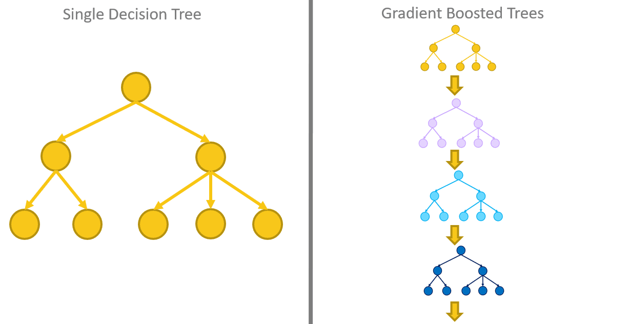
Gradient Boosted Trees

Gradient Boosted Trees are ensemble models combining multiple sequential simple regression trees into a stronger model. Typically, trees of a fixed size are used as base (or weak) learners.

In order to simplify the procedure, regression trees are selected as base learners and the gradient descent algorithm is used to minimize the loss function [5].

Prepackaged Boosting Models

The Analytics Platform offers a few nodes implementing the Gradient Boosted Tree algorithm, based on regression trees. Again, the implementation relies on the Learner-Predictor motif, as for all other supervised algorithms (Fig. 7).

As far as configuration goes, the Gradient Boosted Trees Learner (Regression) node allows the user to set the number of regression trees, the depth of each tree, and the learning rate as the weight to attribute to each tree.

Notice that the Gradient Boosted Tree implementation in The Analytics Platform also contains some elements of the tree ensemble paradigm. Indeed, in the “Advanced” tab of the configuration window, you can set the extraction strategies for the data subset used to train each regression tree.

The Gradient Boosted Trees Predictor (Regression) linearly combines the output of each tree and outputs the final value.

Similarly, the Gradient Boosted Trees Learner and the Gradient Boosted Trees Predictor nodes handle the boosting of the regression trees for classification, interpreting the outputs of the regression trees as class probabilities.

Custom Boosting Models

As for the bagging technique, The Analytics Platform also offers the possibility to customize your boosting strategy with different models than just decision trees. Indeed, The Analytics Platform implements AdaBoost, one of the most commonly used boosting algorithms, with two meta-nodes in the “Mining-> Ensemble Learning” category: the “Boosting Learner” and the “Boosting Predictor” meta-node.

The Boosting Learner meta-node (Fig. 9) implements the learning loop via the Boosting Learner Loop Start node and the Boosting Learner Loop End node.

The Boosting Learner Loop End node sets the maximum number of iterations, the target column, and the predicted column. The target column and the predicted column are used to:

• Identify the misclassified patterns
• Calculate the model error
• Calculate the model weight

The Boosting Learner Loop Start node uses the model weight and the misclassified patterns to alter the composition of the training set.

The loop body includes any supervised training algorithm node, like a Decision Tree Learner or a Naïve Bayes Learner (the default), and its corresponding predictor node. The predictor node is necessary even though this is a learning meta-node because, at each iteration, the identification of correctly and incorrectly classified patterns and the model error calculation are needed.

For each iteration, the boosting loop outputs the model, its error and its weight.

The Boosting Predictor meta-node receives the model list from the Learner node and the input data. For each data row, it loops on all models and weighs their prediction result.

The Boosting Predictor Loop Start node starts the boosting predictor loop by identifying the weight column and the model column (see settings in its configuration window).

The Boosting Predictor Loop End node implements the majority vote on all model results and assigns the final value to the input data row. Its configuration window requires the identification of the prediction column.

The loop body must include the predictor of the mining model as selected in the Learning node.

Conclusions

In this article, we have tried to explain the theory behind the bagging and boosting procedures. We have also shown their most famous implementations, relying on decision trees: Tree Ensembles, Random Forest, and Gradient Boosted Trees.

We have also shown the dedicated nodes and the customizable nodes to train and apply a prepackaged or custom bagging or boosting algorithm in The Analytics Platform.

All examples shown here have been collected in the workflow “Random Forest, Gradient Boosted Trees, and Tree Ensemble” available for free download from the  Hub.

References

[1] L. Breiman. Bagging predictors. Machine Learning, 24:123-140, 1996
[2] Burnham, K. P.; Anderson, D. R. , Model Selection and Multimodel Inference (2nd ed.), Springer-Verlag, (2002)
[3] Tin Kam Ho,Random Decision Forests (PDF). Proceedings of the 3rd International Conference on Document Analysis and Recognition, Montreal, QC, pp. 278–282, 14–16 August 1995
[4] L. Breiman. Random forests. Machine Learning, 45:5-32, 2001
[5] Jerome H. Friedman , Greedy Function Approximation: Gradient Boosting Machine (1999)
[6] Jerome H. Friedman, Greedy Function Approximation: A Gradient Boosting Machine, The Annals of Statistics, Vol. 29, No. 5 , pp. 1189-1232 (Oct., 2001)