
Click to learn more about author Paolo Tamagnini.
In this series, we’ve been exploring the topic of guided labeling by looking at active learning and label density. In the first episode, we introduced the topic of active learning and active learning sampling and moved on to look at label density in the second article. Here are the links to the two previous episodes:
- Guided Labeling Episode 1: An Introduction to Active Learning
- Guided Labeling Episode 2: Label Density
In this third episode, we are moving on to look at model uncertainty.
Using label density, we explore the feature space and retrain the model each time with new labels that are both representative of a good subset of unlabeled data and different from already labeled data of past iterations. However, besides selecting data points based on the overall distribution, we should also prioritize missing labels based on the attached model predictions. In every iteration, we can score the data that still needs to be labeled with the retrained model. What can we infer, given those predictions by the constantly retrained model?
Before we can answer this question, there is another common concept in machine learning classification related to the feature space: the decision boundary. The decision boundary defines a hyper-surface in the feature space of n dimensions, which separates data points depending on the predicted label.
In Figure 1 below, we point again to our data set with only two columns: weight and height. In this case, the decision boundary is a line-drawn machine learning model to predict overweight and underweight conditions. In this example, we use a line. However, we could have also used a curve or a closed shape.
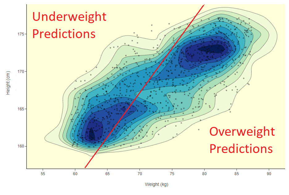
So let’s say we are training an SVM model — starting with no labels and using active learning. That means we are trying to find the right line. We label a few subjects, in the beginning, using label density. Subjects are labeled by simply applying a heuristics called body mass index — no need for a domain expert in this simple example.
In the beginning, the position of the decision boundary will probably be wrong as it is based on only a few data points in the densest areas. However, the more labels you keep adding, the more the line will position itself closer to the actual separation between the two classes. Our focus here is to move this decision boundary to the right position using as few labels as possible. In active learning, this means using as little time as possible of our expensive human-in-the-loop expert.
To use fewer labels, we need data points positioned around the decision boundary, as these are the data points best defining the line we are looking for. But how do we find them, not knowing where this decision boundary lies? The answer is, we use model predictions — and, to be more precise — we use model certainty.
Looking for Misclassification Using Uncertainty
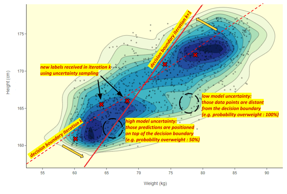
At each iteration, the decision boundary moves when a new point is labeled contradicting the model prediction. The intuition behind model certainty is that a misclassification is more likely to happen when the model is uncertain of its prediction. When the model has already achieved decent performance, model uncertainty is symptomatic of misclassification being more probable, i.e., a wrong prediction. In the feature space, model uncertainty increases as you get closer to the decision boundary. To quickly move our decision boundary to the right position, we, therefore, look for misclassification using uncertainty. In this manner, we select data points that are close to the actual decision boundary (Figure 2).
So here we go. At each iteration, we score all unlabeled data points with the retrained model. Next, we compute the model uncertainty, take the top uncertain predictions, and ask the user to label them. By retraining the model with all of the corrected predictions, we are likely to move the decision boundary in the right direction and achieve better performance with fewer labels.
How Do We Measure Model Certainty/Uncertainty?
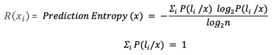
There are different metrics; we are going to use the entropy score (Formula 1 below). This is a concept common in information theory. High entropy is a symptom of high uncertainty. This strategy is also known as uncertainty sampling, and you can find the details in this blog titled Labeling with Active Learning, which was first published in Data Science Central.
Wrapping up
In today’s episode, we’ve taken a look at how model uncertainty can be used as a rapid way of moving our decision boundary to the correct position, using as few labels as possible, i.e., taking up as little time as possible with our expensive human-in-the-loop expert.
In the next blog in this series, we will go on to use uncertainty sampling to exploit the key areas of the feature space to ensure an improvement of the decision boundary. Stay tuned.
This is an on-going series on guided labeling, see each episode at: