
Click to learn more about author Paolo Tamagnini.
One of the key challenges in using supervised machine learning for real world use cases is that most algorithms and models require a sample of data that is large enough to represent the actual reality your model needs to learn.
These data need to be labeled. These labels will be used as the target variable when your predictive model is trained. In this series we’ve been looking at different labeling techniques that improve the guided labeling process and save time and money.
What happened so far:
- Episode 1 introduced as to active learning sampling, bring the human back into the process to help guide the algorithm.
- Episode 2 discussed the label density approach, which follows the strategy that when labeling a dataset you want to label feature space that has a dense cluster of data points.
- Episode 3 moved on to the topic of model uncertainty as a rapid way of moving our decision boundary to the correct position using as few labels as possible and taking up as little time of our expensive human-in-the-loop expert.
Today, We Explore and Exploit the Feature Space
Using uncertainty sampling we can exploit certain key areas of the feature space, which will ensure an improvement of the decision boundary. Using label density, we explore the feature space to find something new the model has never seen before and that might change entirely the decision boundary. The idea now is to use both approaches – label density and uncertainty sampling – at the same time to enhance our active learning sampling. To do this we combine the density score and the uncertainty score in a single metric we can call potential.
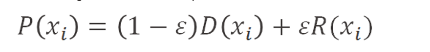
We can now rank the data points that can still be labeled using this potential rank. The epsilon parameter defines which of the two strategies is most contributing. In the beginning, with only a few labels, model performance will be quite bad. That is why it is not wise to use the uncertainty score (R(x) or exploitation). On the contrary the feature space is still unexplored so it makes total sense to leverage on the density score (D(x) or exploration). After labeling for a few iterations, depending on the feature distribution, the exploration strategy will usually become less and less useful as we will have explored most of the dense areas. Despite that, the model should increase in performance as you keep on providing new labels. This means that the exploitation strategy will become more and more useful to finally correctly place the decision boundary. To ensure leveraging on the right technique you can implement a smooth transition so that in the first iterations epsilon is less than 0.5 and when you see an improvement in performance of the model epsilon becomes greater than 0.5.
That is it then, in active learning we can use the potential score to go from exploration to exploitation: from discovering cases in the feature space that are new and interesting to the expert, to focusing on critical ones where the model needs the human input. The question is, though: When do we stop?
The active learning application might implement a threshold for the potential. If no data point is above a certain threshold this means we have explored the entire feature space and the model has enough certainty in every prediction (quite unlikely). Therefore we can end the human-in-the-loop cycle. Another way to stop the application is by measuring the performance of the model if you have enough new labels to build a test set. If the performance of the model has a achieved a certain accuracy we can automatically end the cycle and export the model. Despite those stopping criteria, in most active learning applications the expert is supposed to label as much as possible and freely quit the application and save the output, i.e. the model and the labels gathered so far.
Comparing Active Learning Sampling with Random Sampling
Let’s look at our overweight/underweight prediction example again and do an experiment. We want to compare two SVM models: the first is trained using 10 random data points and the second is trained using 10 data points selected by using the exploration vs exploitation active learning approach. The labels are given by applying the heuristic of the body mass index. If applied to all the rows, such a heuristic would create a curve close to a line which the SVM will try to reproduce based on only 10 data points.
For the random labels approach we simply select 10 random data points, label them “overweight” or “underweight” using the heuristic and then use them to train the SVM. For the active learning sampling approach we will select and label three data points at random and start the active learning loop. We train an SVM and compute the potential score on all the remaining ones. Selecting and labeling the top ranked row by potential, we retrain the SVM with this additional, newly labeled data point. We repeat this a further six times until we have an SVM trained on 10 rows that were selected using active learning sampling. Which model will now perform better? The SVM with randomly picked labels or the model where the labels were selected using active learning sampling?
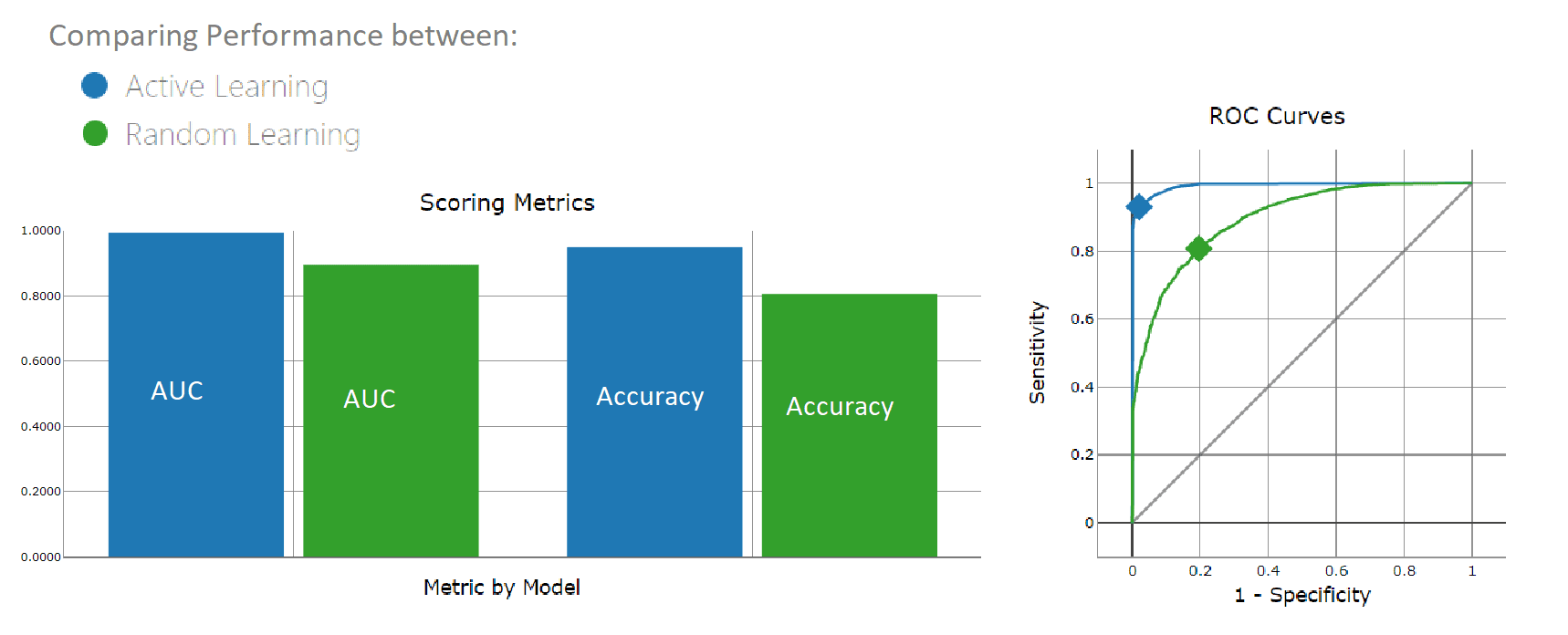
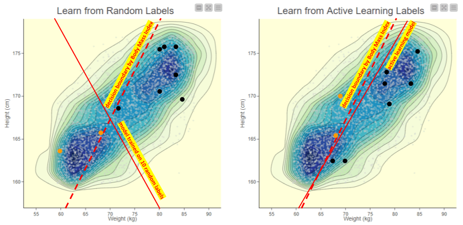
As expected the active learning strategy is more reliable (Fig. 1).The random sampling instead depends entirely on how the 10 data points are randomly distributed in the feature space. In this case they were picked with such bad positioning that the trained SVM is quite distant from the actual decision boundary, found by the body mass index. In comparison, the active learning sampling produces an almost overlapping decision boundary with the body mass index heuristic with only 10 data points. (Fig. 2).
To compute those results we used an Analytics Platform. You can find a workflow (Fig. 3) that runs this experiment on the Hub. It uses the Active Learning Extension. This workflow generates an interactive view (Fig. 3) which you can use to compare misclassifications and the performance of the two models.
The Active Learning Extension provides a number of nodes that allow us to build workflows realizing the active learning technique in various ways. Among these nodes are nodes to estimate the uncertainty of a model, as well as density-based models that ensure that your model explores the entire feature spaces, making it easy to balance exploration and exploitation of your data. You’ll also find a dedicated active learning loop, as well as a labeling view, which can be used to create active learning WebPortal applications. These applications hide the complexity of the underlying workflow and to simply allow the user to concentrate on performing the task of labeling new examples.
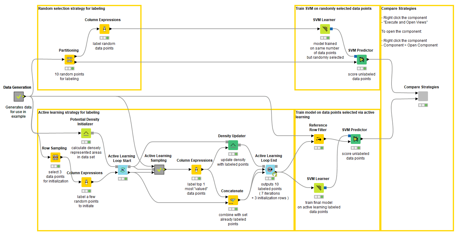
Figure 3. The workflow that runs the experiment. You can download it from the Hub. In the top branch, the partitioning node selects ten random data points to train the first SVM. In the bottom branch, the Active Learning Loops selects ten data points based on the exploration vs. exploitation approach. The predictions of the two models are imported into a component, which generates an interactive view (Fig. 4).
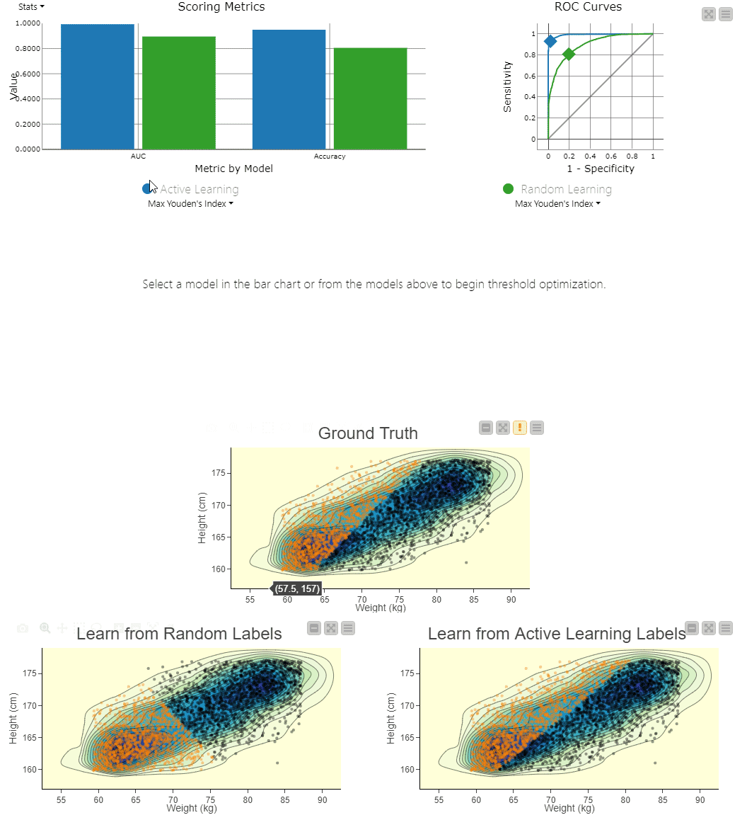
Figure 4. To visually compare the two techniques, the workflow includes a component that generates an interactive view. The view can be used to explore the misclassifications across the two models. You can clearly see the SVM model, which learns from randomly picked labels (bottom left), is classifying quite differently from the actual, ground truth-based decision boundary (center). Using interactivity, it is possible to select data points via the two different confusion matrices and see them selected in the 2D density plots.
Summing up
You now have all the ingredients to start developing your own active learning strategy from exploration to exploitation of unlabeled datasets!
In the next and fifth episode of our series of Guided Labeling Blog Posts we will introduce you to weak supervision, an alternative to active learning for training a supervised model with an unlabeled dataset.
This is an on-going series on guided labeling, see each episode at: